The ancient genomes show many population turnovers
Low-frequency LDA in steppe pastoralist populations: balancing selection in P1 and P2 and its dependence on the locus of mutations
LDA scores around m0 were low when positive selection was achieved in at least one of P1 and P2 and negative selection in P3. There were no abnormal LDA scores found around m0
Stage 2 explored the idea of positive, balancing and negative selection in P1 and P2. The frequency of m0 reached 80%, 50% and 20% when it was positively selected, underwent balancing selection or was negatively selected, respectively, until generation 2,899, when we sampled 20 individuals each in P1 and P2 as the reference samples.
We were able to balance selection at two loci. The positive selection in P1 and P2 made the Mutant allele almost the only one, because of the balancing selection. Positive selection made it possible to get m1 or m2 to reach 80% in P3 unless the all carrier had balance in P1 or P2. If m1 or m2 underwent balancing selection in P3, its frequency slightly increased; for example, if m1 underwent balancing selection in P1, it had a frequency of 25% when P3 was created, and the frequency reached around 37.5% after 20 generations of balancing selection in P3.
Source: Elevated genetic risk for multiple sclerosis emerged in steppe pastoralist populations
Multivariate models for ancestral paths in the ITh genome: The average L2 norm between ancestries at SNPs selected using PALM
LDA thus quantifies the correlations between the ancestry of two SNPs, measuring the proportion of individuals who have experienced a recombination leading to a change in ancestry, relative to the genome-wide baseline. LDA score is the total amount of genome in LDA with each SNP (measured in recombination map distance).
Xrmgd(,j)+Xrm int,j,XrmtgrmLDA
We considered fitting multivariate models by using all the SNPs as covariates. However, the dataset contains only 1,982 cases. Even if only one ancestry is included, the model has 191 predictors, which can result in overfitting problems. Therefore, the GWAS models were preferred to multivariate models.
We were able to use the PALM method to deduce polygenic selection gradients and P values for each trait, in each ancestral path. Full methods and results can be found in Supplementary Note 6.
We define the average L2 norm between ancestries at those SNPs. Specifically, we compute the L2 norm for the ith genome as
We applied the procedure described in ‘HTRX model selection procedure for shorter haplotypes’ for HTRX, HTR and GWAS and visualized the distribution of the out-of-sample R2 for each of the best models selected by each method in Supplementary Fig. 11. In both ‘lm’ and ‘glm’, HTRX had equal predictive performance to the true model. It performed as well as GWAS when interaction effects were absent, explained more variance when an interaction was present and was significantly more explanatory than HTR. The only effective interaction term is rare when rare SNPs are included. In this case, the difference between GWAS and HTRX became smaller, as expected, and removing the rare haplotypes minimally reduced the performance of HTRX.
We started from creating the genotypes for four different SNPs Gijq (where i = 1, …, 100,000 denotes the index of individuals, j = 1 (1XXX), 2 (X1XX), 3 (XX1X) and 4 (XXX1) represents the index of SNPs and q = 1,2 for the two genomes as individuals are diploid). If no rare SNPs were included, we sampled the frequency Fj of these four SNPs from 5% to 95%; otherwise, we sampled the frequency of the first two SNPs from 2% to 5% (in practice, we obtained F1 = 2.8% and F2 = 3.1% under our seed) while the frequency of the last two SNPs was sampled from 5% to 95%. For the ith individual, we used the qth genome of the jth single-syllable polymorphism to take the average value of the two genomes for the ith individual. On the basis of the genotype data, we obtained the haplotype data for each individual, and we considered removing haplotypes rarer than 0.1% or not when rare SNPs were generated. We had 20 fixed covariates, including sex, age and 18 principal components, from UK Biobank for 100,000 individuals.
A random sampling approach for a class of models with significant genetic risk for multiple sclerosis emerged in steppe pastoralist populations. I. Sample selection and the model selection procedure
$${O}{i}=\mathop{\sum }\limits{c=1}^{20}{\beta }{c}{C}{{ic}}+\gamma \left(\mathop{\sum }\limits_{j=1}^{4}{\beta }{{G}{j}}{G}{{ij}}+{\beta }{{H}{1}}{H}{1}\right)+{e}_{i}+w,$$
The model must be fixed with 18 principal components, sex and age and iteratively choose a feature in addition to the fixed covariates to add who can explain the largest variance.
where LM and L0 are the likelihoods for the fitted and null model, respectively. The number of predictors is taken into account and used to determine the adjusted McFadden’s pseudo-R2 value.
$${R}^{2}\left({\rm{SNPs}}\right)={R}^{2}\left({\rm{sex}}+{\rm{age}}+18{\rm{PCs}}+{\rm{SNPs}}\right)-{R}^{2}\left({\rm{sex}}+{\rm{age}}+18{\rm{PCs}}\right).$$
i right and i left, both of which have the same name.
Irmth,rmindividual,rmhas.
Step 1: Select candidate models. The aim of this step is to get more diverse models in order to address the model search problem.
Randomly sample a subset (50%) of data. Specifically, when the outcome is binary, stratified sampling is used to ensure the subset has approximately the same proportion of cases and controls as the whole dataset.
Source: Elevated genetic risk for multiple sclerosis emerged in steppe pastoralist populations
Out-of-Sample Variations in Steppe Pastoralist Populations: Analysis of Outgroup ancestry and SNPs
In each of the ten folds, use a different group as the test dataset and take the remaining groups as the training dataset. In order to compute the additional variations explained by features (out of sample R2) in the test dataset, you must fit all the candidate models on the training dataset. Pick the candidate model with the highest average out-of- sample R2 as the best model.
We performed PCA on the average ancestry probability andWAP at the risk-associated SNPs to sort them into ancestry patterns. 8). The former showed that there was a lot of larger outgroup components in the HLA classes II and III regions. The latter analysis indicated a strong association between steppe ancestry and MS risk. Outgroup ancestry at rs10914539 was found to have a significant effect on the prevalence of the disease, as compared to out group ancestry at RS771767 and rs137956.
Most of the population structure in the UK Biobank 81 can be captured by using 20 predictors from the GWAS models, including sex, age and the first 18 principal components.
The total variation of a trait is explained by the values of the genes, as well as the factors that drive the trait. We computed the variance for each data type in a comparison of the two sets. In this section, we describe the model and covariates accounted for.
We then ran a transformation step as in ref. The Z score is based on the ancestral mean and the centring results. We ran an accelerated bootstrap to get a 95% confidence interval and account for the skew of data to better estimate it.
Source: Elevated genetic risk for multiple sclerosis emerged in steppe pastoralist populations
Dose Distribution of SNPs with Significantly Increased MS Prevalence from Steppe Ancestry Using k-Means Clustering and Gost
$${f}{\left{{\rm{anc}},i\right}}=\frac{{\sum }{j}^{{M}{{\rm{effect}}}}{\rm{painting}}{{\rm{certainty}}}{\left{j,i,{\rm{anc}}\right}}}{{\sum }{j}^{{M}{{\rm{alt}}}}{\rm{painting}}{{\rm{certainty}}}{\left{j,i,{\rm{anc}}\right}}+{\sum }{j}^{{M}{{\rm{effect}}}}{\rm{painting}}{{\rm{certainty}}}{\left{j,i,{\rm{anc}}\right}}},$$
We first applied k-means clustering to the dosage of each ancestry for each associated SNP and investigated the dosage distribution of clusters with significantly higher MS prevalence. For the target SNPs, the elbow method78 suggested selecting around 5–7 clusters, and we chose 6 clusters. The average probability for each ancestry was calculated after we did the k-means cluster analysis. Furthermore, we calculated the prevalence of MS in each cluster and performed a one-sample t test to investigate whether it differed from the overall MS prevalence (0.487%). This tested whether any particular combinations of ancestry were associated with the phenotype at a SNP. Clusters with high MS risk ratios had a high proportion of steppe components (Supplementary Fig. 7), leading to the conclusion that steppe ancestry alone is driving this signal.
The standard deviation is calculated as s.d. We tested the hypothesis (H_0: barpi ) against it.
To test for gene enrichment, we formed a list of all SNPs reaching genome-wide significance (P < 5 × 10⁻⁸) and, using the R package gprofiler2 (ref. 77), converted these to a list of unique genes. We then used gost to perform an enrichment test for each Gene Ontology (GO) term, for which we used default P-value correction via the g:Profiler SCS method. This correction was performed to control the error rate and ensure that all categories are correct.
Source: Elevated genetic risk for multiple sclerosis emerged in steppe pastoralist populations
DNA damage patterns and nuclear contamination in the Archaeobotany of Vestsjlland: the Aalborg Historiske Museum
Authorizations for excavating Kirkegrd, Holbk and Tjrby were granted to the Aalborg Historiske Museum, also known as the Museum Vestsjlland. The current study of samples from those three sites was covered by the agreements that were given to the Globe Institute, University of Copenhagen and Aalborg Historiske Museum.
To determine the authenticity of the ancient reads, post-mortem DNA damage patterns were quantified using mapDamage2.0 (ref. 58). There were two different methods used to estimate the levels of contamination. We applied ContamMix to quantify the number of reads in the mitochondrial reads by comparing the consensus kerchief to possible contaminant kerchief. The consensus was constructed using an in-house Perl script that used sites with at least 5× coverage, and bases were only called if observed in at least 70% of reads covering the site. We applied the ANGSDP to estimate nuclearContamination by measuring Heterozygosity on the X chromosomes in males. Both estimates used a base quality of 20 and a mapping quality of 30.
The data was demultiplexed using a software by illumina called BCL Convert. Adaptor sequences were trimmed and overlapping reads were collapsed using AdapterRemoval (v2.2.4)53. Single-end collapsed reads of at least 30 bp and paired-end reads were mapped to human reference genome build 37 using BWA (v0.7.17)54 with seeding disabled to allow for higher sensitivity. The libraries and lanes were merged with one read per lane, and the duplicate reads were marked using Picard MarkDuplicates. The calculation used all the sites that were used in the calculation and read depth and coverage were determined. duplicates were marked again when the data was merged to the sample level.
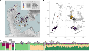
The main population genetics approach on which we based our inference was population-based painting (detailed below). However, to robustly understand population structure, we applied other standard techniques. The first thing we did was analyse the overall population structure of the dataset. The imputed panel had PLINK62 and no SNPs with MAF 0.05. The Medieval and post-Medieval samples clustered close to each other on the basis of 1,210 ancient western Eurasian imputed genomes, displaying a relatively low genetic variability and situated within the genetic variability observed in the post-Bronze Age western Eurasian populations.
57 genome-wide-significant non MHC SNPs for RA were downloaded. We retrieved MHC associations separately (ref. 71; with associated ORs and P values from ref. 72). In total, we created 51 SNPs that were either fine mapped or high in elevation with a fine-mapped SNP.
The data from the 1000 Genomes project had genotypic data of 7,131,965 and whole-genome data of 2,504 individuals.
Analysis of IBD sharing and mixture models were carried out as described3, using the same set of inferred genetic clusters (see Supplementary Data 4). The genetic clustering of the individuals was used to detect IBD segments using IPDseq80 and the network of pairwise IBD sharing similarities. IBD-based PCA was carried out in R using the eigen function on a covariance matrix of pairwise IBD sharing between the respective ancient individuals. We estimated ancestry proportion in supervised modelling of target individuals as mixtures of different sets of putative source groups via non-negative least squares on relative IBD-sharing rate vectors.
Admixture time inference for FBC-associated individuals was carried out using the linkage-disequilibrium-based method DATES44 (HO dataset). The two source groups for the calculation of time for each individual were hunter- gatherer individuals and early farmer individuals.
The predictions of eye and hair colour were made using the HIrisPlex system83. To derive probabilities for brown, blue and grey/intermediate eye colour and blond, brown, black and red hair, we used 18 out of 24 main effect HIrisPlex variants, which have imputed effect allele dosages. We predicted relative ‘genetic height’ using allelic effect estimates from 310 common autosomal SNPs with robustly genome-wide significant allelic effects (P < 10−15) in a recent GWAS of height in the UK Biobank84. The calculated per-sample height polygenic score was for ancient individuals as well as 3,468 Danes from the iPSYCH 2012 case-cohort study. Supplementary note 2 is for more details. Only a fraction of the 100 Danish skeletons were suitable for stature estimation by actual measurement, which is why these values are not reported here.
Bulk collagen isotope values of carbon (δ13C) and nitrogen (δ15N) represent protein sources consumed over several years before death, depending on the skeletal part and the age at death of the individual94,95. Values of 13C and 15N are used to figure out how much marine and tHeretic is used to figure out how much tHeretic is used. Supplementary note 4 is for further discussion. Supplementary Data 2 and Supplementary Note 4 have information on the Stable Ions values from all 100 skeletons and how they were measured. Most of the δ13C and δ15N measurements were conducted at the 14C Centre, University of Belfast according to standard protocols98, based on a modified Longin method including ultra-filtration98,99. Measured uncertainty was within the generally accepted range of ±0.2‰ (1 s.d.) and all samples were within the acceptable atomic C:N range of 2.9–3.6, showing low likelihood of diagenesis100,101.
Strontium isotope analyses can provide a proxy for individual mobility102,103,104. The 87Sr/86Sr ratio in specific skeletal elements may reflect the local geological signature obtained through diet by the individual during early childhood and it will usually remain unchanged during life and after death105. Because of ongoing controversies over the exact use of 106,107, we restrict our observations to patterns that are relative to our own data. Supplementary Data 2 contains the data from the Measurements of 87Sr/86Sr ratios in teeth and petrous bones done at the University of North Carolina- Chapel Hill. For further details see Supplementary Note 5.
We used a pollen diagram from Lake Hjby, Northwest Zealand108, to show how vegetation cover changed during the 5,000–2,400 cal. period. The landscape-reconstruction algorithm is used by bc. At low temporal resolution regional scale, the LRA has previously been applied. 111,112.), and to Iron Age (and later) pollen diagrams113,114, to our knowledge, this is the first time that this quantitative method is applied at local scale to a pollen record spanning the Mesolithic and Neolithic periods in Denmark. In total 60 pollen samples between 6,900 and 4,400 cal. bp were included and the temporal resolution between samples is approximately 40 years. Regional vegetation was estimated with the model REVEALS109 based on pollen data from six other lakes on Zealand (see Supplementary Fig. 6.1 Regional pollen rain and local scale vegetation around Hjby S are calculated from this. Average pollen productivity estimates for Europe115 for 25 wind pollinated species were applied. The reconstructed cover for plant species were then combined into four land cover categories, crops (only cereals), grassland (all other herbs), secondary forest (Betula and Corylus) and primary forest (all other trees). The vegetation reconstruction from Højby Sø is used to illustrate the vegetation development at the Mesolithic/Neolithic transition in eastern Denmark. For more details see Supplementary Note 6.