Post-glacial western Eurasia contains a lot of people

Data analysis of the 1000 Genomes Project: The ancient Danish population and relevant West Eurasian people in the phenomenological setting. II. Downstream analysis

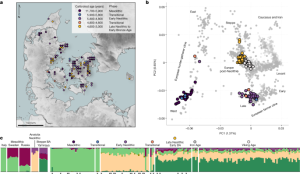
Analyses were based on the 1000 G dataset unless otherwise noted. People not passing the quality control cutoffs were included in the analyses. Four Danish individuals showed possible signs of DNA contamination (Fig. 3 and Supplementary Data 1) and were excluded from most analyses. The multiproxy data they included was included in Fig. 3. Individual metadata for all genetic analyses related to the ancient Danish individuals as well as selected subset of relevant West Eurasian individuals, are reported in Supplementary Data 3.

The allele-frequency-free method was used to infer genetic relatedness. The site-frequency-spectrum approach was used to calculate relatedness estimators for each pair of individuals. We used the realSFS method90 implemented in the ANGSD package91 to infer the 2D-SFS, selecting the SFS with the highest likelihood across ten replicates. We used a set of 1,191,529 autosomal transversion SNPs with MAF ≥ 0.05 from the 1000 Genomes Project36 for the analysis. Previously established cut-offs89 for the KING-robust estimator were applied to assign individual pairs to first-, second- or third-degree relationships. Parent–offspring relationships were distinguished from sibling relationships using R0 and R1 ratios, by requiring that R0 ≤ 0.02 and 0.4 ≤ R1 ≤ 0.6 to infer a parent–offspring relative pair. Individual pairs less than 20,000 in size were excluded.

2,504 people from 26 world-wide populations have whole-genome Sequencing data from the 1000 Genomes project.

To facilitate filtering for downstream analyses, we flagged individuals to potentially exclude according to the following criteria: (i) contamination estimate greater than 5% (‘contMT5pct’, ‘contNuc5pct’; Supplementary Note 1); (ii) autosomal coverage less than 0.1× (‘lowcov’); (iii) genome-wide average imputation genotype probability less than 0.98 (‘lowGpAvg’); (iv) individual is the lower-quality sample in a close relative pair (‘1d_rel’, ‘2d_rel’; Supplementary Note 3c). There were 1,492 individuals that passed all filters, and that was used in most downstream analyses unless otherwise noted.

Analysis of IBD sharing and mixture models were carried out as described3, using the same set of inferred genetic clusters (see Supplementary Data 4). In brief, we used IBDseq80 to detect IBD segments using genetic clustering of the individuals using hierarchical community detection on a network of pairwise IBD-sharing similarities. IBD-based PCA was carried out in R using the eigen function on a covariance matrix of pairwise IBD sharing between the respective ancient individuals. We put ancestry proportion in supervised modelling of targets into a mixture of different sets of source groups using non- negative least squares.

We performed genetic clustering of the ancient individuals using hierarchical community detection on a network of pairwise IBD-sharing similarities103. We ran IBDseq on a dataset restricted to ancient samples only to facilitate the detection of clusters at a larger scale. We constructed a weighted network of the individuals using the igraph104 package in R, with the portion of the genome shared between pairs of individuals as weights. We then performed iterative community detection on this network using the Leiden algorithm105 implemented in the leidenAlg R package (v1.01; https://github.com/kharchenkolab/leidenAlg). We used a resolution parameter of r = 0.5 as the starting value for each level of community detection. If more than one community was detected, we split the network into the respective communities, and repeated the community detection step. If no communities were found, we incremented the resolution parameters step by step until the maximum value was reached. The initial clustering was completed when no more communities were detected at the highest resolution parameter, across all subcommunities. To convert the resulting hierarchy into a final clustering, we simplified the initial clustering by collapsing nodes into single clusters on the basis of observed spatiotemporal annotations of the samples. We note that the obtained clusters should not be interpreted as ‘populations’ in the sense of a local community of individuals, but rather as sets of individuals with shared ancestry. The obtained clusters captured the effects of individuals within restricted areas and/or archaeological contexts, despite the oversimplification of the complex populations investigated here.

Bulk collagen isotope values of carbon (δ13C) and nitrogen (δ15N) represent protein sources consumed over several years before death, depending on the skeletal part and the age at death of the individual94,95. It’s normal to have 13C values as an indicator of the proportion of marine versus terrestrial, and 15N values as an indicator of the trophic level from which the proteins were acquired. Supplementary note 4 is useful for further discussion. Supplementary Data 2 and Supplementary Note 4 discuss the full composition of isotopic measurements, which can be found in all 100 skeletons. The majority of the 13C and 15N measurement were done at the 14C Centre at the University of Belfast according to standard protocols. Measured uncertainty was within the generally accepted range of ±0.2‰ (1 s.d.) and all samples were within the acceptable atomic C:N range of 2.9–3.6, showing low likelihood of diagenesis100,101.

The method DATES 44 was used for the mixture time inference. We estimated admixture time separately for each target individual from Denmark and Sweden, using hunter-gatherer individuals (n = 58) and early farmer individuals (n = 49) as the two source groups.

A proxy for individual mobility can be provided by strontium isotope analyses. The local geological signature obtained through diet can be seen in the 87Sr/86Sr ratio, which will probably stay unchanged during life and after death105. There are ongoing disputes over the exact use of the baseline values106,107, which is why we limit our observations to patterns that are relative to our own data. Measurements of 87Sr/86Sr ratios in teeth and petrous bones were conducted at the Geochronology and Isotope Geochemistry Laboratory (Department of Geological Sciences, University of North Carolina- Chapel Hill) and data are found in Supplementary Data 2. Supplementary Note 5 has more information.

We used a pollen diagram from Lake Hjby to reconstruct the vegetation cover changes during the 5000–2,400 cal. period. The landscape-reconstruction option is being used. The lowest temporal resolution has been the area in which the LRA has been applied. 111,112.), and to Iron Age (and later) pollen diagrams113,114, to our knowledge, this is the first time that this quantitative method is applied at local scale to a pollen record spanning the Mesolithic and Neolithic periods in Denmark. In total 60 pollen samples between 6,900 and 4,400 cal. The temporal resolution between samples is about 40 years. The model REVEALS109 used pollen data from six other lakes on Zealand to estimate regional vegetation. 6.1). Regional pollen rain is calculated using a model called the LOVE model. There were estimates for 25 wind pollinated species. Crops, grassland, other herbs, and secondary forest are all part of the combined cover for plant species. A vegetation reconstruction from Hjby S is being used as a model for the vegetation development at the Neolithic/Neolithic transition. For more details see Supplementary Note 6.