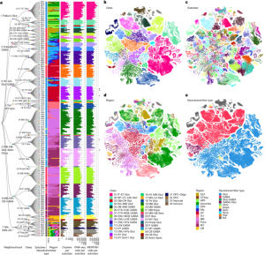
A single-cell analysis of the adult mouse brain is being done

A study of the clustering of open chromatin in snATAC-seq. II. Measurement of the fraction of nuclei detected in the adult mouse brain

No statistical methods were used to predetermine sample sizes. There was no randomization of the samples, and investigators were not blind to the specimens being investigated. The cells were assigned after clustering based on the accessibility of the single nucleus. Potential barcode collisions, as well as low-quality nuclei, were excluded from downstream analysis.

The dataset that we cross-referenced has a comprehensive and annotated brain profile of the adult mouse. Most of the subclass annotations in our data are from the companion study41.

Finally, as snATAC–seq data are very sparse, we selected only elements that were identified as open chromatin in a significant fraction of the cells in each cluster. We selected the same number of non-DHS regions from the genome and used the shuffle function of BEDBedtools to determine the fraction of nuclei for each cell type that showed a signal at these sites. We next fitted a zero-inflated β-model, and empirically identified a significance threshold of FDR < 0.01 to filter potential false positive peaks. Peak regions with FDR < 0.01 in at least one of the clusters were included in downstream analysis. Given one cell subclass, we treat all of the peaks from the subtypes mapped to this subclass as the peaks for the subclass.

Deep Learning on GPUs using Basenji65: a novel loss function for the prediction of chromosome accessibility and mCG methylation

We trained the subclass-level deep-learning model on four NVIDIA A100 80 GB GPUs using the script basenji_train.py from Basenji65. For training, the parameters were set to 32, 150 and 30.

The cell type is represented by the i and j. The matrix is calculated from true signals. The ypred represents the predicted genomic bin-by-type matrix. The pairwise covariance wi,i was calculated between cell types. We then sum the scores across rows and normalize the number of cell types as weights. Last, the weights w was dot multiplied by the original poisson loss.

The model architecture, layers and parameters were adapted from the mouse model, and only the last output head layer had modifications. To encourage the model to predict cCREs in under-represented cell types, we created one novel loss function:

The model was trained on all the subclasses that were annotated. The genome signal tracks were generated with a bigwig format. The training, validation, and testing datasets have been generated using the script basenji_data.py from Basenji65 with the parameters: “-b mm10.blacklist.bed -l 131072 –local -p 16 -t 0.1 -v 0.1 -w 128”.

We used the R package clusterProfiler 100,101 for GO enrichment analysis. The background genes were described in a text before they were selected. The P value was computed using the Fisher exact test and adjusted for multiple comparisons using the Benjamini–Hochberg method.

The signal from the TE-cCREs was aggregated to analyse the variability. To calculate the correlation between chromatin accessibility and mCG methylation in TEs across subclasses, we averaged and normalized the TE-cCRE The companion paper41 gives a signal for each subclass of the TE. To calculate the correlation between chromatin accessibility and RNA expression, we aggregated RNA signals at TE-cCREs of each TE in matched subclasses from a previous study99.

The TE annotation of cCREs was annotated using Homer45 and UCSC mm10 refGene and RepeatMasker annotation. To determine the highTE-cCREs fraction of subclasses we used a mixture model in the R package mixtools97 The P value was calculated based on the null distribution.

Meanwhile, we selected the two peak modules that show global accessibility across the subclasses based on the NMF analysis (Fig. 2f (top left)). We ranked the proximal–distal connections based on their Cicero scores, which were selected after surveying the peak modules above. We performed the Hi-C signals by connecting them to all of the Hi-C data. From the heat maps (Extended Data Fig. 10h), we observed the strong enrichment signals for the global proximal–distal connections.

Exploring the overlaps between ccRXs and FIREs through permutation analysis: A mouse genome study with frequently interacting regions

We tested if cCREs are enriched through permutation analysis. In brief, we shuffled the mouse genome 1,000 times, each time generating 1,053,811 random regions with equivalent sizes as the cCREs. We then calculated the number of overlaps between the randomly generated regions and the FIREs during each shuffle. The number of overlaps on FIREs is more than expected, and that the cCREs are enriched at them.

We applied the criteria in our paper to call out frequently interacting regions in the mouse cortex. The result showed that most FIREs (3,158 out of 3,169) overlap with cCREs in the mouse brain, and a fraction of the cCREs (71,626 out of 1,053,811) overlap with FIREs (Extended Data Fig. 10e).

The coefficient matrix was used to associate modules with cell clusters. Each row is a module and each column is a cluster of cells. The weights of the clusters are indicated by the values in the matrix. The matrix was scaled from 0 to 1 by a column. Subsequently, we used a coefficient > 0.1 (~95th percentile of the whole matrix) as a threshold to associate a cluster with a module.

Grouping cCREs into cis-regulatory modules was done on the basis of relative accessibility across major clusters. NMF was adapted to convert the matrix into a matrix H and a number of modules.

We then retained only reproducible peaks on chromosome 1–19 and both sex chromosomes and filtered ENCODE mm10 blacklist regions. The whole dataset was obtained with the help of a peak list from all of the cell clusters.

We found that, when the cell population varied in read depth or number of nuclei, the MACS2 score varied proportionally due to the nature of the Poisson distribution test in MACS219. It is not possible to do a reads-in-peaks normalization since we do not know how many peaks we will get. To account for differences in the performance of MACS2 based on read depth and/or number of nuclei in individual clusters, we converted MACS2 peak scores (−log10[q]) to SPM37. We took the cut off of 5 into account when determining the peaks that were included in the filter.

To generate a list of reproducible peaks, we retained peaks that (1) were detected in the pooled dataset and overlapped ≥50% of peak length with a peak in both individual replicates or (2) were detected in the pooled dataset and overlapped ≥50% of peak length with a peak in both pseudoreplicates.

We performed peak calling according to the ENCODE ATAC–seq pipeline (https://www.encodeproject.org/atac-seq/) on 1,482 L4-level subtypes and used the same procedure to filter the peaks at both the bulk and single-cell level (Extended Data Fig. As in our previous study19. Before calling peaks, we merged clusters with fewer than 200 cells if they shared the same cell clustering annotations as the L3-level cluster. Next, 1,463 different types were used.

The PCs derived from the previous step were then integrated together using the same method as Seurat v3 through these anchors. The integration step will keep the PCs of the reference dataset unchanged. The resulting PCs from the three datasets were used for t-SNE visualization and k-nearest neighbour (k = 25) graph construction with Euclidean distance. The joint clustering was carried out with the Leiden algorithm on the graph using a resolution of 1.0.

The k-nearest neighbour graph was constructed using the function knn and the method set to kd tree. We next used the function leiden of SnapATAC2 for clustering with the parameter object_function set as modularity. The parameters, which affected the number of clusters a lot, were selected from 0.1 to 2 with a step size 0.1 based on the silhouette coefficients. The resolution of the UMAP 81 was checked to make sure it was in line with the top silhouette coefficients. UMAP projections were calculated using the Python package umap with the parameters a as 1.8956, b as 0.8005 and init as spectral. All of the resolution parameters during clustering are provided in Supplementary Table 3. In our later analysis, we used the term subtypes to represent all of the final clusters from L3-level clustering and L4-level clustering.

We used Scanpy to compute the connectivities over a 20 neighbour local neighbourhood using 250 principal components to build a graph of cell type similarity. We aggregated this weighted adjacency matrix row and column wise by taking the average weights of all cells in a given cell type. We then used the Paris hierarchical clustering algorithm from scikit-network v.0.28.1 to build a dendrogram from our cell type adjacency matrix86. We plotted major cell type markers and examined spatial localization patterns to organize our neuronal clusters into larger sets, comprising a total of 223 groups (metaclusters). Using Scanpy’s rank_genes_groups with the Wilcoxon method, we generated a table of the top 50 differentially expressed genes per metacluster (Supplementary Table 6).

Brain dissections were done in the past. The brains were taken immediately from the 50- to 70 day old mice in the ice cold slicing buffer. CaCl2, 7 mM MgCl2, 1.25 mM NaH2PO4, 110 mM sucrose, 10 mM glucose and 25 mM NaHCO3) that was bubbled with carbogen, and sliced into 0.6-mm coronal sections starting from the frontal pole. From each AAV-retro-Cre-injected brain, the slices were kept in the ice-cold dissection buffer from which selected brain regions (Fig. 1b) were manually dissected under a fluorescence dissecting microscope (Olympus SZX16), following the Allen Mouse Common Coordinate Framework, Reference Atlas, Version 3 (2015; Extended Data Fig. 1). The brain tissues were frozen in dry ice and later stored at 80 C. Only brains that had accurate injections were the subject of dissection. The Olympus cellSens is used for image acquisition.

Experiment on the enrichment of the ATAC-seq accessibility in nucleus libraries using the snmC-sq protocol

The snmC-sq protocol was used to carry out the conversion and library preparation. The libraries were created by barcoded single nucleus samples pooled through two rounds of cleaning and then added to with the use of other amplification methods. Libraries were then pooled, cleaned up with SPRI beads, normalized and sequenced on Illumina Novaseq 6000 using the S4 flow cell 2 × 150 base-pair mode. Illumina MiSeq control software v3.1.0.13 was used for library preparation, as well as Real-Time Analysis v3.4.4 and NovaSeq 6000 control software. Technicians doing nucleus preparations and snmC-seq analyses were blind to the injection sites used for each sample.

The data quality was measured without a required peak set, through the enrichment of ATAC–seq accessibility. We followed a previously described procedure86, and used the function filter_cells in SnapATAC2 to calculate TSS enrichment (TSSe). TSS positions were obtained from the GENCODE87 database v.16. The Tn5 reads were aligned to the positive strand and the negatively aligned ones to the Negative strand, and each of them had a 2,000 tbps relative to each unique TSS genome wide. The profile was normalized to the mean accessibility by smoothing every 11 bp. The maximum was used for the smoothed profile.

It takes more than 1,000 mapped fragments and 10 uniquely mapped fragments to be labeled for each of the 234 samples. The function of the filter_cells was used.

We removed potential doublets for every sample using a modified version of Scrublet28. First, we used the add_tile_matrix function to add the 500 bp genomic bin features, then used the select_features function to filter out the features with frequencies along the samples of lower than 0.5% or higher than 99.5%. We applied the scrublet function to the doublet scores. The parameter expected_doublet_rate was set to 0.08, which is based on our previous experiment on the snATAC–seq pipeline19. Barcodes with scrublet scores of greater than 0.5 were treated as potential doublets and removed from our analysis.

We compared Scrublet with another recently published method named AMULET30, which is used for doublet detection and removal in snATAC–seq data. We simulated datasets containing singlets and artificial doublets from eight samples in the primary motor area and evaluated the performances of the two methods using precision-recall curve (PRC) and area under PRC (AUPRC).

Motif clustering and DMR methylation analysis of mouse mC-RNA co-clusters in SCENIC+

Note that because the GRNs were constructed based only on correlations between data modalities and the binding motifs, they inevitably capture indirect and false-positive relationships. In order to confirm the connections between trans regulators and targets genes,urbation experiments are needed.

We used an ensemble motif database from SCENIC+ (ref. 44), which contained 49,504 motif position weight matrices (PWMs) collected from 29 sources. The clustering ofundant motifs was done by TOMTOM45 and the SCENIC+ authors. There were at least one mouse TF genes involved in the annotated motif clusters. To calculate motif occurrence on DMRs, we used the Cluster-Buster46 implementation in SCENIC+, which scanned motifs in the same cluster together with hidden Markov models.

The unbiased snmC-seq cells from each mC–RNA co-cluster were merged to generate pseudobulk methylation profiles. The epi-retro-seq cells were not used owing to the different genome backgrounds of the mice to avoid confounding results. DMRs were identified within each region group between clusters using ALLCools. We then calculated the PCC between DMR mCG and gene mCH fraction. We used the shuffled genes and DMRs within the sample to calculate the nullPCC and FDR. We used FDR 0.01 to determine the target edges.

To generate the candidate ARGs list, we grouped our pseudocells into 28 groups and assigned the main regions of each to a different excitatory and inhibitory population. The genes of each cell group were calculated using Pairwisegene correlation coefficients across scaled pseudocells from the R package. The correlation of g’s correlations with all genes must be greater than or equal to 99.5% to be considered an ARG candidate. We took selected genes from all cell groups to create a final ARG candidate list.

As we pooled the two mice of the same sex before sequencing, we do not have biological replicates to study the different distribution across clusters of projection neurons from different sexes. We used Fisher tests to identify the difference between males and females but did not take into account the consistency of biological replicates. This could cause false discovery, so we look at the clusters that have no sexual proportion differences to be more confident. We also tested general linear models with binomial dependent variables and use biological replicates as a random effect. The test was biased to identify small clusters because of the limited power for accessing random effects and the number of replicates being too small. Therefore, our dataset provides a general resource across the whole brain suggesting projection-associated cell types, and more biological replicates are needed to validate the patterns and investigate the sexual differences.

Finally, the neurons from each region group were selected and integrated with the scRNA-seq cells from the same region group, using the same procedure as described above. The mC–RNA co-cluster labels were transferred from the scRNA-seq cell to the MERFISH cells. The last step of the MM and DCO subclasses was excluded as the clusters included in the co-cluster analysis were not included.

We note that this could also be achieved through registration of MERFISH DAPI images to the common coordinate framework. However, our companion works demonstrated that the procedure is relatively challenging and it is important to use cell types with known locations as landmarks to refine the registration.

The MERFISH experiments were conducted as described in ref. 17, including the gene panel design, tissue preparation, imaging, data processing and annotation. The dataset includes slices 2, 4, 6, 8, 10, C2, C6, C6, C10, C12 and C14, roughly corresponding to the slices of S1 and S2. The same naming of slices was used throughout the manuscript.

In this manuscript, we only used the absolute proportions, not the relative ones, due to the different profiling strategies between the two datasets. Although the epi-retro-seq samples and unbiased snmC-seq samples were dissected in the same way, we pooled the different dissections into the 32 different sources to carry out FANS and sequencing for epi-retro-seq, so that the proportion of cells from different dissection regions of the same source is likely to follow their proportions in the mouse brain. However, the unbiased snmC-seq profiled all of the dissection regions separately and sequenced the same number of cells in each dissection, which manually amplified the proportion of cells from the smaller or sparser dissection regions relative to the larger or denser ones, and limited the power to estimate the real proportion of neurons in each cluster from the sources.

In QC step 4, the cortical cells from 286 experiments were further filtered to exclude the experiments with a high proportion of neurons of the cell types known not to project to the intended injection site (off-target clusters), using the same method as in our previous study2. Each FANS run we counted the number of neurons that were seen in both known on- and off-target cell types. We compared the observed counts of cells to the counts from snmC-seq data as well as the counts from a sample without projection-type enrichment. The fold enrichment was calculated as. A one-sided exact binomial test was used to determine whether the enrichment of on-target cells was significant. The P value was computed as (\Pr (X\ge {O}{{on}}{;n},p)), in which (X \sim {\rm{binomial}}(n,p)), where ~ represents distributed as,  (n={O}{{\rm{on}}}+{O}{{\rm{off}}}) and (p=\frac{{E}{{\rm{on}}}}{{E}{{\rm{on}}}+{E}{{\rm{off}}}}). For each target, we considered it to be on-target or off-target. The thresholds for FDR were 8 and 0.001. For IT targets, we considered IT as on-target subclasses and layer 6 corticothalamic+inhibitory neurons as off-target. The thresholds were for FDR and fold enrichment. This eliminated 32 out of 286 sorting cases (Extended Data Fig. 2e).

To find anchors between snmC-seq and epi-retro-seq, we used the snmC-seq data to fit a PCA model and use the model to transform epi-retro-seq cells to the same space and find the five nearest snmC-seq cells for each epi-retro-seq cell. In order to find the nearest epi-retro-seq cells for each of the snmC-seq cells we had to fit another PCA model with them. The mutual nearest neighbours between the two datasets were used as anchors and scored using the same method as Seurat v3.

We adopted a similar framework to that of Seurat v3 (ref. 41) for data integration by first identifying the mutual nearest neighbours as anchors between datasets, and then aligning the datasets through the anchors.

Searching for variation in the expression of neurotransmitter genes using a binomial model of cell counts with a non-zero count threshold

The potential doublets were removed in the second part of the process as described in the next section. 2c,d. The information for the cells used in our analysis was based on the type of cells, but we applied more filters to exclude non-neuronal cells and neurons whose projection targets are not confidently assigned.

There would be technical reasons. First, the contamination levels of some experiments might be relatively high, which make larger noise and hinder the models from capturing real projection differences. Different epigenetic differences between different cell types are found across replicates. Third, the sample sizes of some projections are small, which makes learning more challenging. The models are not powerful enough to capture the differences between projections.

Each cell type was assigned to a neurotransmitter identity based upon the percentage of its cells with non-zero counts of genes essential for the function of that neurotransmitter. We used a non-zero threshold.

To identify variable genes, we used a binomial model of homogenous expression and looked for deviations from that expectation, similar to a recently described approach74. The relative bulk expression is computed by summing the counts across cells and dividing by the total UMIs of the population. This is the proportion of all counts that are assigned to that gene. We use this value in a binomial model to observe the genes in cells that have n counts, compared to in a Poisson model. The expected proportion is non-zero counts.

Connecting k-nearest neighbours to distant projections in a brain-wide correspondence of neuronal epigenomics

Assume there are two different datasets in this space, one with labels and one without. We find the k-nearest neighbours in A with a distance that is at least as close as d and then we use d as the weights for the averaged information from the neighbours. After the transformation, the closer neighbours have higher weights, and the weights of all neighbours sum up to 1. To transfer a categorical label from A to B, we used a one-hot encode which represented the label and its vectors in A and B of the query cell. The first part of this is the probability of the query cell belonging to each category. The final assignment uses the category with the maximum probability.

39,461 cells from 519 experiments left were excluded in order to ensure that there was a statistical power of projection analysis. The non-neuronal cells were also removed from the dataset, after which 34,643 neurons remained. The method of cell type classification is explained in the next section.

In quality control (QC) step 1, the cells included in the analysis are required to have a median mCCC level of the experiment < 0.025; 500,000 < nonclonal reads < 10,000,000; and mCCC level < 0.05. In total, 56,843 cells from 703 experiments satisfied these requirements (Extended Data Fig. 2a, b.

Source: Brain-wide correspondence of neuronal epigenomics and distant projections

Iontophoretic injections of rAAV-retro-Cre to stimulate neurons in a granular brain area: Design and experiment, and results for MERFISH

To label the cells projecting to regions of interest with injections of rAAV-retro-Cre. Animals were put into a stereotaxic frame after being anaesthetized with eitherxylazine or isoflurane. Glass micropipettes were used to make the pressure injections of 0.05 to 0.4 l of AAV per injection site. To precisely target PFC, agranular insular cortex, ENT, PIR, AMY, HY and CBN, AAV was injected using iontophoresis to ensure confined viral infection. Iontophoretic injections (+5 µA, 7 s on/7 s off cycles for 5–10 min) were made with glass pipettes with a tip diameter of about 10 μm. For most of the desired target areas, injections were made at different depths, and/or at different anterior–posterior or medial–lateral coordinates to label neurons throughout the target area. More detailed injection coordinates and conditions are listed in Supplementary Table 1. At least two male and two female mice were injected for each desired target. No sample size calculation was carried out. The goal was to get the minimum reproducibility by using two mice of the same sex. Animals used for injections into each brain area were selected at random.

The Salk Institute Animal Care and Use Committee approved all experimental procedures with live animals. The mouse line was kept on the C57BL/6J background. Adult male and female INTACT mice were used for the retrograde labelling experiments. Animals were housed in an Association for Assessment and Accreditation of Laboratory Animal Care-accredited facility at the Salk Institute. Lighting was controlled on a 12 h light/12 h dark cycle. The temperature was adjusted according to the Guide for the Care and Use of Laboratory Animals. Humidity was monitored but not controlled. The animal facilities are surrounded by fresh air which is not recirculated and has the same humidity as the outside air. San Diego has high humidity year-round. The animals were killed 13 days after the operation, and 70 days after the dissection. C57BL/6J ‘wild-type’ mice aged 56–63 days were used for MERFISH experiments.

Gene Set Enrichment Analysis of snRNA-seq Cell Types with MAGMA Z50 and GWAS Summary Statistics

To determine which of our snRNA-seq cell types was enriched for specific GWAS traits, we used scDRS (v.1.0.2)50 with default settings. scDRS uses a single-cell level to calculate disease association scores, and considers the distribution of control genes to identify cells associated with diseases.

We used MAGMA v. 1.10. A window of 10 kb can be used to map single-nucleotide polymorphisms to genes. We used the annotations and GWAS summary statistics to calculate the MAGMA Z score for each gene. Human genes were converted to their mouse orthologs using a homology database from Mouse Genome Informatics (MGI). The 1,000 disease genes used for scDRS were chosen and weighted based on their top MAGMA z scores. The scores from the MAGMA Z50 were used for enrichment, because many traits had previously computed them.

To identify the transcription factors selectively enriched for telencephalic excitatory or inhibitory populations, we performed gene set enrichment analysis (GSEA) on a ranked gene list against a curated transcription factor gene set. First, we ranked genes from our telencephalic excitatory cells by their average correlation with Fos compared with a background ranking of average telencephalic inhibitory Fos correlations. The genes were ranked in chronological order. A set of genes was built with the help of databases from ARCHS4 and TRRUST. We subsetted for human transcription factors that showed up in at least two databases and had at least ten unique targets in each of those databases. The final gene set consisted of these human transcription factors with targets composed of the intersection between any two databases. We used the R package fgsea v.1.20.0 (ref. 100) to run gene set enrichment analysis with a gene set size restriction of 15–500 and against a background of all protein-coding genes expressed in our normalized pseudocell data. P values were computed using a positive one-tailed test and FDR corrected by fgsea.

To identify activity-regulated relationships between our candidate ARGs and regions of the brain, we constructed a force-directed graph of a weighted bipartite network. We built the network with the help of the igraph package which we used to build a matrix of candidate ARGs. An entry e in the matrix represents a correlation between a genes correlation with a brain region that is larger than or equal to one. The nodes of the network comprised two disjoint sets, candidate ARGs and neuronal brain regions, such that there would never be an edge between a pair of genes or a pair of regions. Edges were weighted based on the correlation entry e between a gene and region node. To emphasize the most central nodes in the network, we pruned edges with e less than 1.3. We decided on the core IEGs that should be in the network based on the degree of each of the nodes in the network.

The normalized expression of the pseudocell level of the genes was visualized using a 2nd transformation of the genes. We further normalized the expression of each gene to have a mean expression of zero and a standard deviation of one. For downstream analysis normalized pseudocell counts were used.

We performed reduction of dimensionality at a single cell level to generate pseudocells. The single cells were split into 27 groups based on glial cell classes and neurotransmitter usage. We selected genes for each cell group that were variable in a specific number of mouse donors, so the maximum of 5000 genes would be used for subsequent scaling. We then ran principal component analysis on the scaled expression data (50 principal components for glia and 250 principal components for neurons). Next, we constructed pseudocells by grouping single cells within each cell type. The cells were assigned to pseudocells of size s if the pseudocell size correlated with cell size.

Using scOnline, we aggregated our snRNA-seq expression data into pseudocells: aggregations of cells with similar gene expression profiles. Working at the pseudocell resolution (rather than with individual cells) eliminates the technical variation issues of single-cell transcriptomic data, such as low capture rate from dropouts and pseudoreplication through averaging expression of similar cells93,94, while avoiding issues of pseudobulk approaches, such as low statistical power and high variation in sample sizes95.

To quantify the uncertainty, we calculated the 95% confidence interval for the corresponding binomial distribution using the exact method of binconf function in the Hmisc R package92. For plotting clarity, regions with fewer than five total inhibitory and excitatory cells were excluded.

Each cell type was assigned to an a neuropeptide receptor (NPR) identity if (1) the percentage of its cells with non-zero expression of at least one NPR was greater than or equal to 0.2 and (2) the average expression of at least one NPR was greater than or equal to 0.5 counts per cell.

The NP identity of each cell type was determined by the percentage of cells with non-zero expression of the NP and average expression of the NP. Four NPs showed greater contamination across other cell types, including OXT, which is a subclass of PM CH. We required the percentage of cells with non-zero expression to be greater than or equal to 0.8 and the average expression to be more than five counts per cell for these NPs.

For the 166 neuronal cell types that did not meet the above nz conditions, we carefully examined their top expressing transporters and assigned neurotransmitters accordingly.

Source: The molecular cytoarchitecture of the adult mouse brain

A Mixed Integer Linear Programming Model for Cell Type Dendrograms in Deep CCF Regions: Application to Immunity, Projection and Cerebellum

To find the minimally sized gene lists that allowed us to distinguish one cell type from the others in the dataset, we framed the question as a set covering problem. In the set cover problem, we find the smallest subfamily of a family of sets that can still cover all the elements in the universe set. We can define this as a mixed integer linear programming model programmatically using the JuMP domain-specific modelling language in Julia (refs. There is 33,89. We optimized using the HiGHS open-source solver (v.1.5.1)90 or the IBM ILOG CPLEX commercial solver v.22.1.0.0 (ref. 91). Supplementary Methods has the mixed integer linear programming model derivation and CPLEX solver parameters used.

To generate the neighbourhood ridge plots in Fig. In Supplementary Table 13, we identified the interneuron and projection metaclusters for the isoculum, striatum and cerebellum. Supplementary Table 5 shows the cell types within each metacluster.

To generate the force-directed graph of regional cell type similarity, as in Fig. We weighted the DeepCCF regions according to the weighted Jaccard similarity metric. We used qgraph to create a force-directed graph.

To assess cluster heterogeneity across regions with vastly different areas, we analysed the minimum number of cell types required to cover 95% of the mapped beads. For each region, we computed the number of confidently mapped beads for each cell type sorted in descending order by the number of beads. The number of cells necessary for the running sum of beads was determined after we had mapped all the beads.

Descendants from more distant ancestors were aggregated in order to find the neighbourhood of the index cell type. We continued aggregating until the number of cell types in the neighbourhood would surpass 100 or for neurons, if the next set of cell types was more than 60% non-neuronal.

The genes and cell types were initially reordered using the R package slanter’s default permuting method87. The cell types were then reordered to comply with the cell type dendrogram structure using a dynamic programming tree-crossing minimization optimization88.

The leaf sequence in the tree was improved by changing the order of the children of the internal nodes. We did so by iteratively permuting the columns and rows of a normalized cell type by gene matrix so that the elements are grouped around the diagonal. The genes were picked for their ability to carry Dlx1, Lhx, Foxg1, Lhx8, Lhx8, and Gata3.

RCTD in doublet mode models how well explicit pairs of cell types match a bead’s expression. For computational efficiency, RCTD prefilters which cell type pairs are considered per bead. However, we were able to map fine-grained cell types because of the larger cell type references, but due to the lack of prefiltering, we were unable to find many similar cell types. To balance this sparsity, we added an additional ridge regression term to RCTD’s quadratic optimization tunable with a ridge strength parameter, which allowed us to control the relative sparsity and potential overfitting of the prefiltering stage. Our modified prefiltering stage used a heuristic to detect a subset of potential cell types for each bead by using RCTD’s full mode with two ridge strength parameters (0.01, 0.001), as well as mapping each cell type individually.

We modified RCTD scores so that we can aid in mapping large references with many similar clusters. We identified the cell type pairs that were similar to the best- scoring pair because we didn’t use the result of single-cell type pair that fit best. We took the total occurrences of all cell types and divided them into well-fitting pairs to come up with a confidence score. For a map with a confidence threshold of at least 0.25, we use a maximum score of 0.2.

In accordance with the explicit cell type pairs used within RCTD’s doublet mode, we subdivided this filtered list, pulling out the 10 cell types deemed most likely to be associated with the given bead. We used only the cell types from the top 10 and the rest of the prefiltered list in modelling how well these cell types mapped to a bead. The amount of cell types considered for the cerebellum was very low, and we were able to use all pairs to run the scheme.

OSQP 81 scales better for the larger matrices because of larger cell types being mapped, and this is why we changed the programming of RCTD. We also rewrote the inner loops of the most time-intensive functions (choose_sigma_c and fitPixels) with Rcpp82 for efficiency. Additionally, we used Hail Batch (refs. 83,84) and GNU Parallel85, which allowed for large-scale, on-demand parallelization (to thousands of cores) using cloud computing services.

Source: The molecular cytoarchitecture of the adult mouse brain

Systematic Identifying and Removal of Excluded Immune Cell Clusters in the snRNA-Seq Data using the SCOPIT Package

We identified 16 cell classes in our snRNA-seq data, 6 of which were excluded from the majority of our analyses (dendritic cell, granulocyte, lymphocyte, myeloid, olfactory ensheathing and pituitary). Most of these excluded clusters are classified as immune cell types and are mentioned in the following figure and tables: Extended Data Fig. 1a,d,h and Supplementary Tables 2 and 3. We were able to identify immune cell populations.

We used the SCOPIT package to estimate the saturation of our data. Under the prospective sequencing model, SCOPIT calculates the multinomial probability of sequencing enough cells, n, above some success probability, p, in a population containing k rare cell types of size N cells, from which we want to sample at least c cells in each cell type:

Next, we constructed a cell ‘quality network’ to systematically identify and remove remaining low-quality cells and artefacts from the dataset. By simultaneously considering multiple quality metrics, we have increased power to identify low-quality cells, while skirting issues related to setting hard thresholds on multiple quality metrics. To construct the quality network, we considered the following cell-level metrics: (1) per cent expression of genes involved in oxidative phosphorylation; (2) per cent expression of mitochondrial genes; (3) per cent expression of genes encoding ribosomal proteins; (4) per cent expression of IEG expression; (5) per cent expression explained by the 50 highest expressing genes; (6) per cent expression of long non-coding RNAs; (7) number of unique genes log2 transformed); and (8) number of unique UMIs (log2 transformed). We constructed separate quality networks for both glial and neurons. The quality network was clustered using a shared nearest neighbour and Seurat clustering. The strategy was to take any clusters out of the network, so that they had alier distribution of quality metric profiles. A distribution of quality metric was considered as an outlier if its median was above 85% of cells in three features of the quality network: oxidative phosphorylation, mitochondrial and ribosomal protein expression. We further removed any remaining clusters with fewer than 15 cells.

For visualization with high-dimensionality. 1a, we first subsampled each of the clusters to a maximum of 2,000 nuclei. Using the Scanpy package, we calculated the first 250 principal components of our subsampled cells. To generate a t-SNE we used a perplexity of 350 and an inflated factor of four on the principal component space.

The only exception to the above was if the next level of clustering resulted in a set of differential clusters that passed this test; these were situations where the first round of clustering split the cells on a continuous difference in expression but the next round resolved the discrete clusters. These clusters can be subclustered if they contain additional structure.

The leaves were considered when testing for differential markers. We used a Mann–Whitney U-test to assess whether any genes are differentially expressed. As an additional filter, we required that a gene be observed in less than 10% of the lower population and observed at a rate at least 20% higher in the higher population to ensure that there is a discrete difference in expression between the two populations. We required every cluster to have at least three marker genes distinguishing it from its neighbours as well as three marker genes in the other direction. If a cluster failed that test, all leaves were merged, and the parent was considered the terminal cluster.

If the resolution sweep concluded at the highest resolution without ever finding multiple clusters, this is also indicative of a homogenous population, and clustering was considered completed.

There is no resolution low enough to form a single cluster if the shared neighbour graph is not a single connected component. This would typically occur if there were very few variable genes, which is indicative of a homogenous cell population.

Once we computed the shared nearest neighbour graph, we used the Leiden algorithm to identify cell clusters using the Constant Potts Model for modularity77. This method is sensitive to a resolution parameter, which can be interpreted as a density threshold that separates intercluster and intracluster connections. The sweep strategy was implemented to find the relevant resolution parameters. We started with a very low-resolution value, which results in all cells in one cluster. We slowly increased the resolution until there were at least two clusters, and at least 5% of the cells weren’t in the largest cluster. Any cluster of fewer than (\sqrt{N}) cells was discarded, where N was the number being clustered in that round. This discarded set constituted roughly 1.6% of the total cells (100,280 of 5.9 million).

The graph75, 76 was constructed after selecting variable genes. After transforming the counts with the square- root function, we computed the k-nearest neighbour (kNG) graph using the coefficients (k50) and cosine distance. From the kNN graph, we compute the shared neighbour graph, where the weight between a pair of cells is the Jaccard similarity over their neighbours:

We compared this expected value with the observed percentage of non-zero counts and selected all genes that are observed at least 5% less than expected in a given population.

The genes Dsp,Ccn2 and Tmem212 were analysed to find out which parts of their expression correspond to CCF regions in Supplementary Table 12.

For ease of visualization, we grouped the CCF hierarchy into 12 ‘main regions’: isocortex, olfactory areas (OLF), hippocampal formation (HPF), striatum (STR), pallidum (PAL), hypothalamus (HY), thalamus (TH), midbrain (MB), pons (P), medulla (MY) and cerebellum (CB). Many of our analyses included a section called ‘DeepCCF’ regions, detailed in the Supplementary Table 4.

Source: The molecular cytoarchitecture of the adult mouse brain

Joint alignment of a large deformation diffeomorphic metric mapping dataset with a gradient-based approach using Reimannian gradient descent

This dissimilarity function, subject to Large Deformation Diffeomorphic Metric Mapping regularization, is minimized jointly over all parameters using a gradient-based approach, with estimation of parameters for linear transforms accelerated using Reimannian gradient descent as recently described71. The source code for the standard registration pipeline is available online at https://github.com/twardlab/emdmm. The annotations were drawn onto each slice using the transformations above. The boundaries of each anatomical region were rendered as black curves and overlaid on the imaging data for quality control. We visually inspected the alignment accuracy on each slice and identified 15 outliers, where our rigid motion model was insufficient owing to large distortions of tissue slices. We included an additional two-dimensional diffeomorphism to model distortion that are independent from slice to slice and cannot be treated as a three-dimensional shape change. The data was extended. 2a shows accuracy before and after applying the additional two-dimensional diffeomorphism.

An objective function, called previously 69,70, was developed by us to measure the differences between the transformed atlas and our dataset after we transformed the contrast of the atlas to match the color of our Nissl data. To transform contrasts, a third-order polynomial was estimated on each slice of the transformed atlas to best match the red, green and blue channels of our Nissl dataset (12 degrees of freedom per slice). During this process, outlier pixels (artifacts or missing tissue) are estimated using an expectation maximization algorithm, and the posterior probabilities that pixels are not outliers are used as weights in our weighted sum of square error.

For each puck, we created a greyscale intensity image from theSlide-seq data by summing the UMI counts at each bead location on the puck and making a normalized image. We then performed the alignment of these images to the adjacent Nissl images in two steps. First, we transformed each Nissl image to an intermediate coordinate space using a manual rigid transformation. The aim of this first transformation was to bring the images to an upright orientation, making the second step of alignment easier. In the second step, we manually identified corresponding fiducial markers in the Nissl images and Slide-seq intensity images using the Slicer3D tool v.4.11 (ref. 66) along with the IGT fiducial registration extension67. Using the fiducial markers, we used thin-plate spline interpolation to get bead positions and the parameters that went with them.

The beads were matched between the sequence of reads and the sequence of the read to get the same Gene Count matrix.

Source: The molecular cytoarchitecture of the adult mouse brain

Nissl Images on an Olympus VS120 Microscope Using the Pike 505C VC50 Camera and Slide-seq Pipeline for the Study of the Lower Spinal Brain

We acquired Nissl images on an Olympus VS120 microscope using a ×20, 0.75 numerical aperture objective. Images were captured with a Pike 505C VC50 camera under autoexposure mode with a halogen lamp at 92% power. The pixel size in all images was 0.3428 μm in both the height and width directions. We acquired a total of 114 Nissl images, each from an adjacent section of the brain to a corresponding section that was processed using the Slide-seq pipeline. We removed 10 from the lower spine that were outside the CCF reference brain in the 114 sections. We removed three sections because of the poor quality of the corresponding data. The remaining 101 images comprise the final dataset that we use for all our analyses.

Slide-seq arrays were generated as previously described2 with slight modifications. The larger-diameter gaskets were used to make the bead array. These sizes were chosen to facilitate different anterior to posterior coronal section sizes. The amount of digital binning that was utilized was 1.3 m per pixel.

Sequencing reads were demultiplexed and aligned to a GRCm39.103 reference using CellRanger v.5.0.1 using default settings (except for an additional parameter to include introns). We used CellBender v.3-alpha63 to remove cells contaminated with ambient RNA.

Source: The molecular cytoarchitecture of the adult mouse brain

Laboratory animal care procedures for the BRAIN: BICCN protocol 0120-09-16. The blood cell population in mouse brain studied by Isoflurane anaesthesia

The C57BL/6J mice were anesthetized by administration of isoflurane in a gas chamber for 1 min. The negative tail pinch response was confirmed by Anaesthesia. Animals were moved to a dissection tray, and anaesthesia was prolonged with a nose cone flowing 3% isoflurane for the duration of the procedure. The Transcardial Perfusions were done with an ice-cold pH 7.4 HEPES buffer. NaCl, 10 mM HEPES, 25 mM glucose, 75 mM sucrose, 7.5 mM MgCl2 and 2.5 mM KCl to remove blood from brain and other organs sampled. The meninges were removed from the brain and frozen in liquid nitrogen for 3 min before being cooled to 80 C for long-term storage. For use in generation of the Slide-seq dataset through serial sectioning, the brains were removed immediately, blotted free of residual liquid, rinsed twice with OCT to assure good surface adhesion and then oriented carefully in plastic freezing cassettes filled with OCT. The cassettes were forced to be vibrated for 5 minutes at a room temperature in order to remove air bubbles and adhere to the brain surface. The brain’s precise orientation in the x–y–z axes was then reset just before freezing over a bath of liquid nitrogen vapour. Frozen blocks were stored at −80 °C.

Animals were group housed with a 12-h light–dark schedule and allowed to acclimate to their housing environment (20–22.2 °C, 30–50% humidity) for 2 weeks post-arrival. All laboratory animal care procedures were approved by the Massachusetts Institute of Technology Committee on Animal Care in accordance with the US National Institute of Health guide for the care and use of laboratory animals. All procedures involving animals at the Broad Institute were conducted in accordance with the US National Institutes of Health Guide for the Care and Use of Laboratory Animals under protocol number 0120-09-16.

BICCN researchers mapped these cell types into the mouse brain. Advancements in these genomic technologies allowed the team to catalogue 90% of cell types in the adult mouse brain in two years. The NIH has launched another five-year project called the BRAIN Initiative Cell Atlas Network, with the aim of scaling up the technologies to map the brain cell types of humans and non-human primates, as well as the mouse brain, during the organ’s development.

The BICCN was funded by the National Institute of Health to the tune of US$372 million and has been working with 250 scientists at 45 institutions.

The Korea Brain Initiative is looking at several scales in the brain, including the prefrontal cortex and the basal ganglia. The same technologies being utilized by the NIH and the China Brain Project are being used by its researchers.

The European Union’s Human Brain Project, which was located in Switzerland, created the Human Brain Atlas. This can be found on the HBP’s open platform. The atlas uses post-mortem brain-imaging data and depicts the multilevel organization of the brain, from its cellular and molecular architecture to its functional modules and neural connections.

After nearly 20 years, the Swiss Blue Brain Project will wrap up its work with the release of a digital model of the mouse brain.

Towards data standardization and classification of cell clusters in zoo: a unified approach to cell classification, classification and classification

As the projects progress, there is a need for better communication between them. Several of the projects are using similar or identical technologies. It makes sense for the teams to liaise more closely, at the very least to begin a discusson on how to establish shared data standards, which they have not yet done.

At a minimum, the data, models and code need to be open. Complying with large data sets such as these remains a challenge. A framework for data collection and analysis, including definitions for types of cell clusters as well as unified cell classifications and names across species, will eventually be needed.