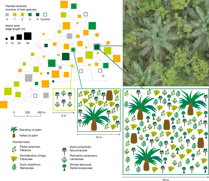
Oil palm landscapes have tree biodiversity islands

Measurement of above-ground biomass, biomass and microclimate using a combined thermal camera and a thermal camera on a multicopter drone

Miccolis, A., van Noordwijk, M. & Amaral, J. in Tree Commodities and Resilient Green Economies in Africa (eds Minang, P. A., Duguma, L. A. & van Noordwijk, M.) Ch. 27 (World Agroforestry, 2021); available at https://go.nature.com/3jfvuq9

We measured the diameter at the breast and the tree’s height a year ago for all the trees. In January and February 2017, we also measured the height of the oil palms at meristem, that is, the point of attachment of the young leaves to the oil palm trunk30. We estimated above-ground biomass of the trees (equation (5)) and the oil palms (equation (6)) using the respective allometric equations of refs. 90,91:

We used a multicopter drone to record land and canopy surface temperatures using a thermal camera attached to a TeAx ThermalCapture module. 94. Each plot was covered once over a 9 day period, with image sets being recorded four to five times per day. The main input for modelling heat transfer in W m2 was the land and canopy surface temperatures. Measured short-wave radiation and relative humidity were used as further input variables to support the prediction of latent heat flux and derive evapotranspiration.

We measured the microclimate using temperature per humidity loggers. The loggers were installed in the middle of each plot at 1.5 m above ground and were protected from water and direct solar radiation using handmade multiplate radiation shields97. The data was collected for a year from 18 November to 19 September. The time is between midnight and 3 h. We calculated the daily amplitude using the absolute difference between the values as a proxy for microclimate buffering.

Fungal community analysis using Illumina next-generation sequencing: ITS2 marker region. Assessment and taxonomy of OTUs in January 2017

In January 2017 three soil cores (10 cm depth, 4 cm diameter) were taken within each 5 × 5 m2 subplot. The surface leaf litter had to be removed. The roots were separated from the soil after it was sieved. The fungal community was assessed using Illumina next-generation sequencing (Illumina) of the ITS2 marker region. The protocol for amplification, amplicons and generation of Otu is detailed in the ref. There was 65. OTUs were classified taxonomically using the BLAST (blastn, v.2.7.1) algorithm66 and the UNITE v.7.2 (UNITE_public_01.12.2017.fasta) reference database67.

Source: https://www.nature.com/articles/s41586-023-06086-5

Measurement of the Structural Complexity of Understorey Vegetation. I. Ground Covering, Oil Palm and Tree Density

The variables we measured are representative of the vegetation structure. We used a terrestrial laser scanner Focus M70 (Faro Technologies) to create three-dimensional point clouds of the vegetation at the centre of each plot in September and October 2016, as described in ref. 30. The stand structural complexity index was computed by us. 99 and its two components: (2) the mean fractal dimension index (MeanFRAC) derived from cross-sections of polygons in the three-dimensional point cloud, which is a scale-independent and density-dependent measure of structural complexity and (3) the effective number of layers (ENL) that describes vertical stratification based on the Simpson Index100. The three measures were derived from vegetation parts over 130 cm. In order to measure the structural complexity of the understorey vegetation, we derived the understory complexity index that measures the fractal dimensions of horizontal cross-sections of the point cloud between 80 and 180 cm height. (5) Canopy gap fraction was estimated from hemispherical photographs at plot level as described in ref. 30. The canopy was further partitioned by drone-based photogrammetry in October 2016 as a result of the oil palm and tree cover. There is a file with the names of all the people We also used the drone-based orthophotos to calculate (8) oil palm density as the number of living oil palms per plot irrespective of the orientation of the plot relative to the planting scheme (Supplementary Figs. 2 and 3) . For the smaller plots (5 × 5 m) unaffected by thinning, the oil palm density was simply the typical planting density in conventionally managed oil palm plantations (120 planted palms per hectare). The oil palm density calculation is given in the Supplementary Note 3. We also calculated (9) tree density as the number of trees planted and from natural regeneration per plot and expressed per hectare. We estimated the portion of the ground (in percent) as (10) understorey vegetation cover and (11) litter cover per subplot in February–March 2018. The understorey vegetation cover included all parts of plants lower than 130 cm in height, including the trunks and other parts of the planted trees but excluding oil palm trunks. The mean value of the litter depth was measured in 3 randomly chosen positions inside each subplot by using a metal ruler. We applied a principal component analysis to all the structural variables after they were standardized to zero mean and unit variance.

We derived taxonomic diversity for soil bacteria and soil fungi, soil fauna, herbs, trees, seeds, pollen, understorey arthropods, birds and bats. Most of the groups (arthropods, herbs, trees, birds and seeds) were sorted at the lowest possible taxonomic level (species or morphospecies). Pollen, soil fauna and bats were sorted to higher levels, mainly family, order and morphotypes, respectively. Soil bacteria and soil fungi were analysed by DNA-based marker gene sequencing as amplicons sequence variants or OTU, respectively. Hereafter, we refer to these different taxonomic units (species, family, order, morphotypes and OTU) as ‘species’ for simplicity.

The trees were surveyed in the first and second months of the year. Furthermore, we surveyed all free-standing woody plants (trees, shrubs and bamboos) that colonized the plots with a length of ≥130 cm from April until August 2018. For each species or morphospecies, one voucher specimen was collected, dried and pressed according to standard procedure. In the main text, we refer to the colonized woody plants as ‘trees’, unless stated otherwise. Because the number of sampled trees largely varied according to the tree island area, we standardized the diversity estimates using rarefaction curves (R package iNEXT)82 to 24 individuals, which represent the median number of individuals per plot.

Multidiversity and multifunctionality were used to calculate the indicators of biodiversity and ecosystems functioning. Following ref. 18, we performed a cluster analysis to preselect indicators for achieving a representative measure of ‘ecosystem function multifunctionality’. As tree growth and litter input were correlated and formed a cluster, we excluded tree growth from the analysis (Supplementary Note 4 and Supplementary Fig. 4). Following a threshold approach108, we calculated multifunctionality (and multidiversity) as the number of ecosystem functioning (and biodiversity) indicators that cross a threshold, expressed as a certain percentage of the maximum observed values in our study landscape (among all 56 study plots). In the main text we presented results for a 50% threshold for all thresholds, from 1% to 99%. To reduce the influence of extreme values, we used the mean of the three highest values observed in all study plots, respectively. As an alternative to the threshold approach, we also calculated multidiversity and multifunctionality as the average of the indicators108. Before multidiversity and multifunctionality calculations, all the variables were standardized to unit scale (for biodiversity and ecosystem functioning separately). The calculations were performed using the package multifunc in R108.

Source: https://www.nature.com/articles/s41586-023-06086-5

Measurement of saturated soil hydraulic conductivity using a dual-head infiltrometer in the 35 subplots of conventionally managed oil palm monocultures

Researchers from Indonesia included in the research process included design, study implementation, data ownership, intellectual property and authorship of publications. Local and regional research relevant to our study was considered in citations.

To quantify soil water infiltration capacity, we measured saturated soil hydraulic conductivity (Kfs, cm h−1) using a dual-head infiltrometer (Saturo) in March 2018 near the subplot centre in 35 (out of the 52) tree islands and in the four control plots representing conventionally managed oil palm monocultures. A broken instrument meant the 17 remaining plots were measured with a manual double-ring infiltrometer that tends to yield more estimates than a dual-head approach. The Kfs were measured in three plots. We plotted these values against each other and found a close linear relationship (R² = 0.98, P = 0.066); even though it was only marginally significant because of the small sample size, we used it to correct the values from the 17 plots that were measured manually (Kfs_corr = 1.44 + 0.55 Kfs_double_ring) to allow for comparability across all 56 plots.

There were 20 litterbags, each filled with 12 g of material and made from palm fronds and air-dried leaf litter. In each plot, one litterbag was installed in November of last year. The difference between the initial litter dry mass and litter dry mass remaining after 6 months was calculated to be the amount of material lost.

The values were aggregated using the median per plot of the litter weight. We excluded outliers defined as plot-level values outside of the range of 3 standard deviations from the entire data (less than 5% of the litter weight data, total and per species). To get annual estimates, we summed the available plot-level values over time and divided them by the number of sampling dates (that is, between 17 and 24, depending on the number of missing traps or excluded outliers). The values obtained by the seed trap area were used to get the leaf litter fall.

Source: https://www.nature.com/articles/s41586-023-06086-5

EFForTS Core Plot Analysis of the Peronema Canescens Wood Density based on Local Areas of Plots

$${{\rm{B}}{\rm{A}}}{{\rm{i}}{\rm{n}}{\rm{c}},2017-2018}=\sum ({{\rm{B}}{\rm{A}}}{{\rm{t}}{\rm{r}}{\rm{e}}{\rm{e}},2018}-\sum {{\rm{B}}{\rm{A}}}_{{\rm{t}}{\rm{r}}{\rm{e}}{\rm{e}},2017})/A.$$

dpalm, density of oil palms, is the number of oil palms per ha and takes into account the local neighbourhoods of the plots.

rmArmGrmB_rmtrmr.

Wood density for Peronema canescens was based on a plot data of the EFForTS core plot. (0.36 g cm−3), Shorea leprosula (0.44 g cm−3) and Durio zibethinus (0.516 g cm−3) it was taken from the global wood density database92.

$${Y}{{\rm{F}}{\rm{o}}{\rm{r}}{\rm{e}}{\rm{g}}{\rm{o}}{\rm{n}}{\rm{e}}}={N}{{\rm{f}}{\rm{e}}{\rm{l}}{\rm{l}}{\rm{e}}{\rm{d}}}\times {Y}_{{\rm{p}}{\rm{_}}{\rm{r}}{\rm{e}}{\rm{f}}}$$

Source: https://www.nature.com/articles/s41586-023-06086-5

Extension of the Behling Pest Control Plane to the Field Sites of C. annuum (Canadian Pseudomonas)

We assessed pollination rate on chilli pepper plants (Capsicum annuum) as phytometer plants, selected for potential shade tolerance87, widespread home garden cultivation in this region88 and the potential role pollination can play in fruit quality and yield89. 1,500 individuals of a local variety of C. annuum were raised from seed outside of the plots. The NPK was applied at the field sites after the local practices to standardize growing conditions and control pest damage had been practiced. We halted fertilizer and pesticide application 1 week before placement in the plots and only watered as conditions required thereafter. In February of this year, we selected 204 individuals to transfer to the 56 study plots. The four chilli Plants were placed, still in their pots, at the centre of each plot for 5 weeks for open pollination and monitoring and three weeks for fruit harvesting. We removed any flowers before placement in the field, so pollinated flowers and developing fruits were assumed to result from pollination within the study plots. Each plot was refreshed once per week and the number of flowers were counted per plant before the final harvest. To calculate the rate of successful pollination, you need to divide the total number of harvests by the number of flowers seen per plot.

From June until October, the Behling pollen traps were installed to collect rain. Each trap has a plastic tube which is placed 30 cm above the ground and holds a pole. The mosquito net on the top of the tube prevents the cotton from being removed and reduces the amount of animals or litter that gets into the tube. It is necessary to prevent the pollen from pouring out of the trap in tropical countries when there are heavy rains. glycerol has a higher density than water, which is used in the Behling trap. The rain can flow out of the trap without the pollen, which is trapped in the synthetic cotton and glycerol83. The traps had been changed to mimic the environment. The plots had 168 pollen traps installed. The traps were not recovered in three of the 56 plots. One pollen trap from each 53 plot was processed and analysed. The pollen traps were washed with water and then sieved to remove the large amount of materials. Afterwards, the pollen traps were sieved through a 150 µm mesh sieve to exclude medium-sized materials from the samples. Two LYCOPodium tablets were added to each sample to estimate palynomorph concentrations 84 and the same was done to remove cellulose material. Residues were mounted for use in a pollen visualization and identification program. Light microscopy was used to carry out analysis of the peckle and the spore. The pictures of all the identified pollen and spore types were taken with a photomicroscope. For each trap, a total sum of at least 100 pollen grains were counted. It is difficult to identify the pollen and spore grains at species level and the level of identification varies for different groups of plants. Consequently, a reduction to the family level has been proposed for studies involving analysis of palynological diversity in the tropics86.

All non-woody terrestrial vascular plants (for example, angiosperm herbs and vines, ferns, but not epiphytes) in the subplot were recorded from February until March 2018. They were classified to species or morphospecies and herbaceous cover (in absolute per cent ratios from 1% to 100%) was estimated by two people. Epiphytes that grow on the leaves of trees or palms are not included. vine species that grow in the ground and climb up trees are included. Herbarium specimens were collected and stored in the laboratory of Jambi University. The names were checked after The Plant List 2013, v. 1.1 ( http://www.theplantlist.org).

We installed four seed traps in each of the 56 study plots for 1 yr, that is, between 1 April 2017 and 29 March 2018. The traps were built using fine-mesh cloth attached to a squared structure made in PVC pipes of size 50 cm × 50 cm fixed at 1 m from the ground. The traps were installed at random locations in each of the four quadrants of each plot, at a minimum distance of 1 m from the plot edge. The traps had to be dried at 40 C for 3 days. All the seeds were carefully extracted from the samples, counted and separated by morphospecies using hand lenses (×10 magnification) and a microscope (Leica photomicroscope with ×400 magnification) for very small seeds. Molecular identification of the morphospecies was implemented using three universal plant DNA barcodes (matK, rbcL and ITS2)75,76,77,78 and taxonomic assignments were made using BLASTn search against the NCBI Genbank reference sequence database79. The barcode sequence were deposited in the Genbank under the same accession numbers as the others. We used available literature in order to classify each morphotype as a native or non-native species. We derived the native seed density (number of native seeds per m2) as the total number of native seeds over the entire sampling duration per plot, which was used as an indicator of ecosystem functioning (see ‘Ecosystem functioning’). Seed diversity, calculated on the basis of the Hill number frameworks and used as indicators of biodiversity (see ‘Biodiversity’), was derived from the pooled samples per plot over the entire sampling duration for all seeds (native and non-native).

Three core of the topsoil were taken in May of 2017). The soil core was mixed and released from the roots. A total of 5 ml of RNAprotect Bacteria reagent (Qiagen) was added to 5 g of soils to prevent nucleic acid degradation. DNA and RNA were extracted from 1 g of soil by using the Qiagen RNeasy PowerSoil Total RNA Kit and the RNeasy PowerSoil DNA Elution Kit (Qiagen). The 16s ribosomalRNAGene was amplified and mapped as described in ref. The quality of the pairs was checked by fastp and merged with PEAR. (ref. 70). The last primer sequence was clipped with cutadapt v. 2.5. There were several things done with vsearch, including size filtering, dereplication and chimaera removal. 72). The sequence was then mapped against a database of SILVA’s. Counts were normalized by using the GMPR normalization74.

During October–November 2016, in each plot, four soil samples of 16 × 16 cm2 were taken randomly within the subplot with a spade. There are samples of litter and soil up to a depth of 5 cm. Animals were extracted using a gradient heat extractor61 and collected in dimethyleneglycol–water solution (1:1) and thereafter transferred into 70% ethanol62. All animals were counted and categorized into 28 groups, which are allowed for functional group classifications. All animals that are classified as detritivores, herbivores and predator in the sample were calculated by means of community metabolism estimates derived from ref. 63. The estimates are based on measurements of more than 5,000 individuals of soil animals across eight different oil palm plantations in the same region; to estimate community metabolism, individual body masses were recalculated to metabolic rates using group-specific regressions from ref. 64. Community metabolism was calculated by summing up metabolic rates of all individuals; we used the mean per plot across four samples for each functional group (detritivores, herbivores and predators) for the analysis. The number of taxonomic groups in each plot was used to calculate the total number of diversity.

Arthropods were sampled in the understorey vegetation during October 2016 to January 2017. Each plot was sampled three times with six pan traps per plot exposed for 45 h. Traps were made of white plastic soup bowls covered with yellow ultraviolet spray-paint53 and were filled with water and one drop of regular soap. They were fixed in a holding system in groups of three at the height of the surrounding plants and these systems then equally distributed in distance from edge and to each other. All arthropods were preserved in 70% ethanol. All individuals were identified as belonging to higher morphospecies. The taxonomic groups Hymenoptera, Lepidoptera and Araneae were categorized into functional groups (pollinators, predators and parasitoids) using different identification keys54,55,56,57,58,59,60 (Supplementary Table 10). Predators and parasitoids were merged into the single functional group ‘predators’.

We used an acoustic SMX-ii microphone on the left channel and a full spectrum Sonitor Parus49 microphone on the right, strapped to wooden poles at a height of 1.5 for the recording. We use sound recordings to get sound samples of birds and bats. We used two stereo 15 min recordings starting 15 min before sunset and two 15 min stereo recordings starting at sunrise, sampled at 22.05 kHz for birds. We used two 40 min mono sound recordings from the right channel, extracted from consecutive nights, starting 20 min after sunset, sampled at 384 kHz for bats. Twelve sound recorders were installed at the same time. The recordings were annotated in ecoSound-web50 to extract their duration, bat pass and bird detection distances. Birds were assigned to species according to Birdlife International. Owing to the lack of standard protocols and reference collections for Southeast Asia, we could not identify bats to species and used sonotypes instead. All bats were echolocating and so were considered insectivorous bats, thus the appended feeding guild information. Only bird vocalizations detected within a 28 m radius were included, which corresponds to the diameter of the largest study plot (40 × 40 m2). We used the maximum number of individuals detected simultaneously in all recordings per plot as a conservative proxy of abundance per bird species or bat sonotype.