There are 140,000 people from Mexico City
Multivariate Analysis of SNPs in the Mexican Aboriginal X-ray Binary, ABCA1 Variances and the Linkage Disequilibrium Scale
The leaders of the Indigenous communities and the National Commission for the Development of Indigenous Communities of Mexico (CDI), have approval of the individuals that have been recruited into the MAIS cohort. All participants gave their consent and authorities and community leaders assisted with the translation. The consent form described how findings from the study may have commercial value and be used by for-profit companies. Sample collection for MAIS was approved by the Bioethics and Research Committees of the Insituto Nacional de Medicina Genómica in Mexico City (protocol numbers 31/2011/I and 12/2018/I). The data from the MAIS cohort has been discussed with the Indigenous leaders and volunteer individuals included in the study to explain the meaning of the findings and the possibilities for using the data in future collaborations.
Such regions are useful for our analyses only in so much as they reflect demographic and environmental histories that may affect the genetic and complex trait variation we are interested in. We consider ancestral variations within such regional groupings in several analyses, as well as the origins and implications of this scale to discretize at, and we carry out changes in the scales within such groupings.
ABCA1 variant frequencies were computed using plink in individuals from the MXB stratified by ancestry proxies from ADMIXTURE or by HDL cholesterol levels (Supplementary Fig. 59).
For each reference panel, we restricted the analysis to autosomes, removed all monomorphic SNPs, flipped all SNPs to the forward strand, and removed SNPs with an ambiguous strand.
We chose not to do linkage disequilibrium analyses given the large loss of SNPs in Mexican admixed people. We repeated the analysis on a set of SNPs pruned for linkage disequilibrium and obtained similar results (data not shown). Given the admixed nature of Mexicans, we didn’t remove SNPs from the MXB because they were expected to be out of the Hardy–Weinberg equilibrium.
We also include two random predictors in our model. These are: the covariance structure defined by the genetic relationship matrix; and the locality where the individual is from to capture any other environmental variation (such as diet) not captured by the fixed predictors.
A random sample of 4,000 people had their GWAS done, as described above. For quantitative traits, raw values were again normalized within the selected subset before analysis.
Indigenous Population Control and Population Analysis in Two Medieval City Regions of Mexico: Coyoacn and Iztapalapa
Biometric data were filtered to remove outliers with apparent errors in data entry. The height and weight of outliers ranged from 100 cm to 300 cm and were based on distribution density.
Blood pressure was manuallycurated for people whose values differed by more than 20 units for the two readings, as well as people with values that were high or low. Both readings were manually checked, and discordant readings were discarded. The remaining samples were merged with the updated values. A set of blood pressure phenotypes were adjusted to correspond with treatment for hypertension. In those individuals who were reported to be receiving some form of hypertension treatment, 15 units were added to systolic blood pressure and 10 to diastolic blood pressure (SBP_adj and DBP_adj)53,54.
We have access to data for a lot of these factors including access to healthcare, clean water and yearly income, as well as whether or not they speak an Indigenous language.
Localities were assigned values of latitude, longitude and altitude (metres) using data from the National Institute of Statistics and Geography (INEGI) in Mexico.
There were randomly selected areas within the two cities to recruit participants. The districts are close to the ancient Aztec city of Tenochtitlan, and have been since the pre-Hispanic period. The population dynamics have changed over the centuries but original Indigenous populations settled there. The capital of New Spain was being constructed over the ruins of Tenochtitlan, and a number of people from Spain resided in Coyoacn. The populations of Coyoacn and Iztapalapa derive largely from the migration from the 1950s to the 1970s. Over this period, both districts, but particularly Iztapalapa, received large numbers of Indigenous migrants from the central (Nahuas, Otomies and Purepechas), south (Mixtecos, Zapotecos and Mazatecos) and southeast (Chinantecos, Totonacas and Mayas) regions of the country.
gnomAD v.3.1: a reference dataset outside low-complexity regions for comparison with the MCPS WES data
We downloaded the gnomAD v.3.1 reference dataset, which we retained high-quality variant annotations, as well as low-complexity SNVs, outside low-complexity regions. We additionally overlapped gnomAD variants with TOPMed Freeze 8 high-quality variants (FILTER=”PASS”) (https://bravo.sph.umich.edu/freeze8/hg38). We further merged gnomAD variants and MCPS exome variants by the chromosome, position, reference allele and alternative allele names and excluded MCPS singletons, which were heterozygous in ancestry. This process resulted in 2,249,986 overlapping variants available for comparison with the MCPS WES data. Median sample sizes in gnomAD non-Finish Europeans, African/Admixed African and Admixed American populations were 34,014, 20,719 and 7,639, respectively.
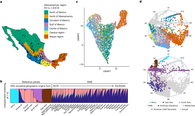
smartpca from Eigenstrat62 was used to carry out the PCA. Principal components generated by smartpca (Supplementary Figs. 6 and 7) were used to carry out the uniform manifold approximation and projection (UMAP) analysis (Fig. 1c and Supplementary Figs. 19 and 20)63. FST analysis was carried out using smartpca.
A Computational Method to Estimate the Mutation Burden of Diverse Populations using Admixture Bayes and Matrix Stats
Mutation burden is defined as the sum of derived alleles carried by an individual. A computational pipeline using vcftools, python, linux and R was used to compute mutation burden in different classes of variants, and at different derived allele frequency thresholds. We computed either a rare mutation burden (derived allele frequency ≤ 5%) or an overall mutation burden considering all allele frequencies. The R packages matrixStats, dplyr and ggplot2 were used. We correlated the mutation burden with the global ancestry percentage from different present-day continental origins in all individuals. The ancestry estimates were from the admixture analysis. We did a Spearman’s correlation and P value calculation.
Using AdmixtureBayes, we inferred the split events and admixture events that have occurred in the MXB. We used the default parameters for generating the admixture graph with the exception of the number of chains and iterations, which we set to a higher value of 16 (–MCMC_chains 16) and 20,000 (–n 20000) to ensure convergence; we also used the -slower flag, enabling the computation of the necessary information to plot the top trees, and a burn-in period corresponding to half the samples. The tree was plotted with the highest probabilities to show a representation of inferred admixture events. The AdmixtureBayes method and prior used details can be found in the corresponding paper.
Source: Mexican Biobank advances population and medical genomics of diverse ancestries
Variant Effect Predictors for FUMA SNP2GENE in the Minimal X-Ray Baryon Population (MXB)
ROH were also correlated with birth year in the MXB (Fig. 3b) It was used as a variable in the analysis. For the birth year analysis, we removed the first two decades, as each year has below 15 individuals sampled in this period. Birth year was also directly correlated with ancestries from the Americas (inferred using ADMIXTURE) in rural and urban localities separately. The ancestries per individual estimated from the admixture analysis were correlated with the ROH (fig. 3a and supplementary fig. 32). An R script was used to analyse the distribution of the sum of ROH by geography.
The functional effects of the variant were determined by whether or not they were derived or ancestral. Ancestral alleles for each SNP in the MXB were inferred using the EPO pipeline from the 1000 Genomes Project. The Variant Effect Predictor was used to pick one consequence (or transcript) per variant according to a criterion that included the canonical status of the transcript, APPRIS isoform annotation and transcript support level.
The lead association SNPs were defined using FINEMAP (v.1.2.1; R2 = 0.7; Bayes factor 2), which was based on the summary statistics for each of the associated traits. FUMA SNP2GENE was then used to identify the nearest genes to each locus on the basis of the linkage disequilibrium calculated using the 1000 Genomes EUR populations, and explore previously reported associations in the GWAS catalogue40,71 (Supplementary Table 7).
In the late 1990s, a meeting between scientists from the UNAM and the University of Oxford resulted in the establishment of the MCPS. These discussions evolved into a plan to establish a prospective cohort study that could investigate not only the health effects of tobacco but also those of many other factors (including factors measurable in the blood)1. More than 100,000 women and 50,000 men who were older than 50 years old agreed to take part in the study and were asked questions about their health and agreed to be tracked for cause-specific mortality. More women were recruited because study visits were made during working hours when women were more likely to be at home, although visits were extended into the early evenings and weekends to increase the proportion of men in the study.
The MCPS 10k reference panel: DNA phenotyping and phasing using phased WGS and wnbgS data
A blood sample from each participant was collected and sent to a central laboratory using a transport box chilled with ice packs. The samples were kept refrigerated overnight at 4 C, then were separated the next morning. After being stored at 80 C for a bit, the samples were taken to Oxford for long-term storage over liquid nitrogen. The UK Biocentre has a buffy coat, which was used to extract DNA from it. Some samples provided a minimum of 1.5 g DNA at 10 ng l but the majority of samples yielded 2 g DNA at a 20 ng l concentration.
Approximately 250 ng of total DNA was enzymatically sheared to a mean fragment size of 350 bp. 10 bp barcodes were added to the DNA fragments after ligation of a Y-shaped adapters. Libraries were quantified with quantitative PCR, pooled and then analyzed using 150 bp pair-end reads with two 10 bp index reads on the Illumina NovaSeq 6000 platform. A total of 10,008 samples had their fingerprints taken. This included over 150 mother– father–child trios. The rest of the samples were chosen to be unrelated to third degree or closer and enriched for parents of nuclear families. 99% of samples had an average coverage of 30 while all samples had an average coverage of 27.
We took the support-vector- machine-filtered WES and wnbgS datasets and put them on the array scaffold. The phased WGS data constitute the MCPS10k reference panel. The information we got from the sequence reads and from the subset of available trios and pedigrees was fed into Shapeit. The 100,000 and 10,000WES chunks were used for phasing with 500 SNPs from the array data to start and end each chunk. The use of a phased scaffold meant that chunks of data could be concatenated together to make a whole file, preserving the phasing of array variant. When a variant appeared in the array and Sequencing datasets, the data from the array dataset was used.
Similar to other recent large-scale genomes, we implemented supervised machine-learning to discriminate between high- and low-quality samples. In brief, we defined a set of positive control and negative control variants based on the following criteria: (1) concordance in genotype calls between array and exome-sequencing data; (2) transmitted singletons; (3) an external set of likely ‘high quality’ sites; and (4) an external set of likely ‘low quality’ sites. To form the external high-quality set we first created the intersection of the two genes that passed QC. This set was additionally restricted to 1000 genomes phase 1 high-confidence SNPs from the 1000 Genomes project36 and gold-standard insertions and deletions from the 1000 Genomes project and a previous study37, both available through the GATK resource bundle (https://gatk.broadinstitute.org/hc/en-us/articles/360035890811-Resource-bundle). To define the external low-quality set, we intersected gnomAD v3.1 fail variants with TOPMed Freeze 8 Mendelian or duplicate discordant variants. An equal number of variant were kept in the positive and negative labels across the different frequencies after the control set of variant was binned. A support machine using a radial basis function was trained on up to 33 available site quality metrics, including, for example, the median value for allele balance in heterogeneous calls and whether a variant was split from multi-allelic sites. We split the data into training (80%) and test (20%) sets. We used cross- validation to identify the hyperparameters that returned the highest accuracy in the training set, and applied them to the test set to confirm accuracy. This approach identified a total of 616,028 WES and 22,784,866 WGS variant as low-quality, of which 161,707 and 104,450 were coding variant. We further applied a set of hard filters to exclude monomorphs, unresolved duplicates, variants with >10% missingness, ≥3 mendel errors (WGS only) or failed Hardy–Weinberg equilibrium (HWE) with excess heterozgosity (HWE P < 1 × 10–30 and observed heterozygote count of >1.5× expected heterozygote count), which resulted in a dataset of 9,325,897 WES and 131,851,586 WGS variants (of which 4,037,949 and 1,460,499 were coding variants, respectively).
We used Shapeit (v.4.1.3; https://odelaneau.github.io/shapeit4) to phase the array dataset of 138,511 samples and 539,315 autosomal variants that passed the array QC procedure. To improve the phasing quality, we leveraged the inferred family information by building a partial haplotype scaffold on unphased genotypes at 1,266 trios from 3,475 inferred nuclear families identified (randomly selecting one offspring per family when there was more than one). We then ran Shapeit one chromosome at a time, passing the scaffold information with the –scaffold option.
If no error is committed, each maximal haplotypes is descended from a common ancestor. The edges are going to be missing due to mistakes made in IBD calling. Set of connected components is what we see. Because we limited edges to pairs of third-degree relatives or closer, we assumed missing edges in connected components are false negatives and included them. We removed edges between haplotypes that were observed to have different alleles.
IBD segments from hapIBD were summed across pairs of individuals to create a network of IBD sharing represented by the weight matrix (W\in {{\mathbb{R}}}{\ge 0}^{n\times n}) for n samples. Each entry gives the total length of the genome, which individuals i and j share by descent. The low-dimensional visualization was created to show off the IBD network. We used a similar approach to that described in ref. The eigenvectors of the normalized graph Laplacian were used for a low-dimensional embedding of the IBD network. Let D be the degree matrix of the graph with ({d}{{ii}}=\sum {{j}}{w}{{ij}}) and 0 elsewhere. The normalized (random walk) graph Laplacian is defined to be (L=I-{D}^{-1}W), where I is the identity matrix.
Source: Genotyping, sequencing and analysis of 140,000 adults from Mexico City
Accuracy of the imputation assessment using a mixture of imputed and masked genotypes in the WES data
We measured imputation accuracy by comparing the imputed dosage genotypes to the true (masked) genotypes at variants not on the arrays. Markers were binned according to how they looked in the samples. In each bin, we report the squared correlation (r2) between the concatenated vector of all the true (masked) genotypes at markers and the vector of all imputed dosages at the same markers. Variants that had a missing rate of 100% in the WGS dataset before phasing were removed from the imputation assessment.
mathopsum limits_i=1,p,
An estimate of the effective sample size for population k at the site is ({n}{k}={{\rm{AN}}}{k}/2). The sites can be hard to phase using current methods. Family information and phase information in sequencing reads was used in the WGS phasing, and this helped to phase a proportion of the singleton sites. In the WES data we found that over half of the exome singletons occurred in stretches of their families’ancestry. We gave the same weight to the two ancestries when estimating allele frequencies for these variants.
$$\begin{array}{l}{V}{l}\,=\,{{(i,j)}{l}:{\rm{for}}\,1\le j\le 2\,{\rm{and}}\,1\le i\le N}\ {E}{l}\,=\,{({(i,j)}{l},{(s,t)}{l}):{h}^{{(i,j)}{l}}\,{\rm{and}}\,{h}^{{(s,t)}_{l}}\,{\rm{are}}\,{\rm{IBD}}}.\end{array}$$
N equals sum Cin C_rmALTbar.
Source: Genotyping, sequencing and analysis of 140,000 adults from Mexico City
Impact of sex and ancestry on the Performance of the Population Prediction Model in the Presence of Discriminant Disorder (MCPS)
The regression of theBMI values by sex and ancestry was used to evaluate the performance of the PRS. As for the generation of summary statistics, individuals with diabetes were excluded from the analysis. Incremental R 2 was used to reduce the sum of squares error between models. The model was used to estimate the effect-size estimates for the rawBMI values, as well as the age, sex, and ancestry. Two approaches were used to assess the impact of ancestry differences on source summary statistics. For the MCPS, individuals were divided into quantiles by estimated Indigenous Mexican Ancestry using the LAI approach described above. The metrics were calculated using the 1000 Genomes-based continental ancestry of the UK Biobank.