The recovery of European freshwater flora has come to a halt
Indicators of Freshwater Invertebrate Communities: Taxonomic and Functional Biodiversity Metrics in a Two-Step Approach
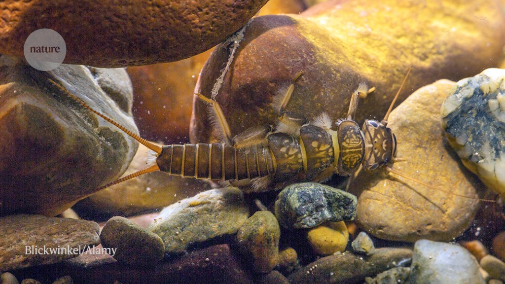
We calculated taxonomic and functional diversity metrics representing freshwater invertebrate communities across sites and over time. We looked at native and non-native species as well as insects and EPT taxa, which are grouped as an indicator of water quality.
Temporal trends in each taxonomic (abundance, richness, Shannon’s diversity, Shannon’s evenness, individual-based rarefied richness and temporal turnover), functional (redundancy, richness, evenness, turnover, divergence and Rao’s quadratic entropy) and community subset (taxon richness and abundance of native species, non-native species, EPT taxa and insects only) metric were assessed using a two-step approach. We used R to calculate the site-level trends for each metric. The temporal trend estimate was represented in the models by the coefficients of the continuous predictor and the metric biodiversity.
We assessed the responses of the climate metrics and the land cover values for the sample period, as well as the impact score and sub catchment characteristics. We did not include upstream land-use trends as most sites exhibited low variation: cropland cover changed by a mean of −0.002% per year ± 0.11 s.e.m., with no change detected at 634 sites; urban cover changed by 2.48% per year ± 0.14 s.e.m., but with no change detected at 803 sites. To look at relationships between environmental drivers and biodiversity trends, we models trend estimates using an LMM and include trend errors for the calculation of the overall trend, as well as study identity and country as random effects.
The form was brm and it was used for the moving window trend estimate.
Using brms80, we modelled the effect of year on moving-window trends to see if there is a linear change in the trajectory.
We calculated the proportion of the total L MM intercept above and below zero, which is the probability of an increase or decrease in the mean trend.
We ran linear mixed-effects models (LMM) in the brms package to synthesize site-level data and estimate overall mean trends. The LMM included site-level trend estimates as the response, and an overall intercept and two random effects (country and study identity) as predictors. Random effects accounted for data heterogeneity because there are more sites in some countries. We assumed normal errors because the site-level trends were normally distributed. The mean trend across studies has been estimated using a meta-analysis model that combines site-level trends with uncertainty from the s.d.
Community Uniqueness, Divergence and Land Cover Predictions in the TerraClimate Dataset from 1992 to 2020 Using the R Package
We calculated six distance-based metrics to be used to describe multiple aspects of community niche space and align them with the other diversity metrics. The function in the R package was used to calculate all functional metrics. In calculations of functional richness and divergence, we used six principal coordinate analysis axes (the dbFD ‘m’ argument), according to current recommendations67. To enable calculation of functional turnover, we calculated community-weighted means of each functional trait category weighted by taxa abundance, then calculated turnover of the community-weighted means using the R package codyn, as for taxonomic temporal turnover57,68. We calculated abundance-weighted functional redundancy using the unique function in the package. The value of community uniqueness has been calculated as a function of Simpson diversity and functional redundancy, as 1 U. The trait input matrix was based on Euclidean distances bound between 0 and 1 and the tolerance threshold was 10−8.
Fixed-year variables were centred to improve model convergence (cYear) and year in the temporal autocorrelation term was included as a count with the first year of sampling considered year 1 (iYear). The models accounted for the residual temporal autocorrelation by using an ar(1), day of year and additional predictor when there was variation in sampling dates greater than 30 days.
We calculated the proportion of land cover categories in each subcatchment using the ESA CCI Land Cover time series81 for each year from 1992 to 2018. Land cover data is available for almost all of the sites analysed. We used the r.water.outlet module to calculate the total amount of each point occurrence and the percentage cover of the land categories within this area. The areas of cropland and urban land were calculated as the percentage of the upstream area averaged across the sampled years at each site.
We extracted monthly climatic predictors from the TerraClimate dataset79 for 1967–2020, which covered all sites and years. We identified the sampling month and computed the mean monthly climatic value for each site. Cumulative annual precipitation and maximum monthly temperature are predictors of cumulative annual precipitation andmaximum monthly temperature at each site. The trend values in precipitation and temperature were calculated using models that were fitted with the R package. The models used to calculate site-level biodiversity metric trends were similar to the models used to estimate the coefficients of a continuous year effect. The Terra Climate dataset is associated with uncertainty in some areas, but we have a large number of sampling sites, good station coverage and a low complexity of most site locations.
Source: The recovery of European freshwater biodiversity has come to a halt
A Detailed Spectroscopic Analysis of the 90m Digital Stream Network Using the MERIT Hydro75 Digital Elevation Model
The MERIT Hydro75 digital elevation model allows us to see the peaks and valleys in the high resolution Hydrography 90m stream network. To achieve a high spatial accuracy, we used an upstream contributing area of 0.05 km2 as the stream channel initialization threshold. We next calculated the subcatchments for each segment of the stream network, that is, the area contributing laterally to a given stream reach between two nodes, using the r.basins module. The location of a site is not always visible due to inaccuracy of the DEM or the coordinates. To ensure that point occurrences matched the DEM-derived stream network and therefore the network topology, we first identified the subcatchment in which each point occurrence was located, then moved all points to the corresponding stream segments using the v.net module within the given subcatchment. From each point, we calculated the network (as the fish swims) distance (km) using the v.net.distance module, and the Euclidean (as the crow flies) distance to all other point occurrences using the v.distance module. The distance was set when sites weren’t connected through the network because they were in different drainage basins.
In total, we identified 61 non-native species. The first analysis of native and non-native species was limited to 1,299 sites in which taxa were identified to the species or mixed resolution, which did not allow for reliable identification of non. Estimates of trends in non-native species richness and abundance were restricted to the 898 (of 1,299) sites at which non-native species were recorded. The two non-native species that were most abundant were the New Zealand mud snail and the North American bladder snail.
We took the following steps to fill in gaps due to missing trait data. First, when trait data were not available at the original identification level (15.9% trait coverage across taxa), we used genus-level trait data, resulting in 48.2% coverage. Genus-level trait data are generally sufficient to represent most interspecific variation among freshwater invertebrates and thus taxon responses to environmental variability61. Next, we replaced missing values in the trait modalities with the median of the trait profiles from the full taxons of the species we were identified to in order to achieve 61.3% coverage. 90.5% of the taxa was covered when we replaced missing values in trait data with the median value of trait profiles of all genera within a family. The lack of accurate phylogenies for many invertebrate taxa, a low trait coverage at the species level and mixed genotypic resolution across sampling sites prevented the use of other gap filling approaches, but taxonomic aggregation usually agrees with expert trait assignments.
Our compiled time series represent different stream types and stream orders from a large geographical area of Europe. Detailed information about the purpose of the data is not available for some time series. These data were not selected randomly but were collected from available studies that met our six criteria. We can’t rule out biases from sites that have different impact levels from those that have the least impact as the data was collected from sites that were exposed to differing levels of impact.
Between 13 and 509 taxa were collected in all of the years. Communities from 42% of sites were identified to species, 30% were identified to mixed (species-to-family) taxonomic levels and 28% were identified primarily to family. There were 2,694 taxa from 959 genera, 212 families and 47 groups. We list time-series locations, durations and characteristics in Supplementary Table 2 and list the number of sites sampled per year and country in Supplementary Table 3.