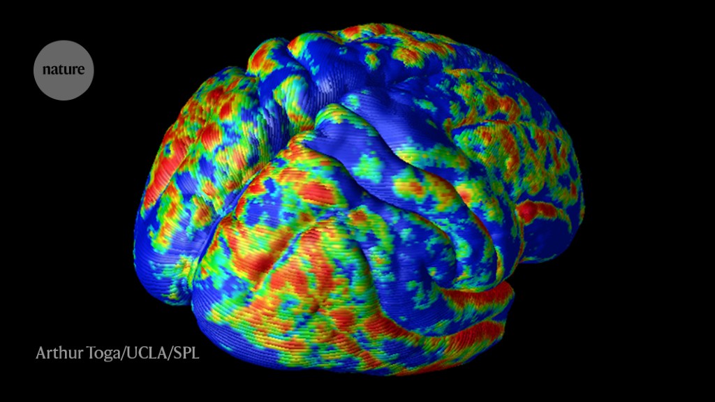
Geometric constraints on brain function
A subcortical atlas for the generation of a mask in a hemisphere. I. Basic modes for waves of vibrations
The first method for generating a mask in each hemisphere was done with the Harvard–Oxford subcortical atlas. Voxels with a probability of 25% or more of belonging to these structures were included in the masks. We used FreeSurfer’s mri_mc function and the Gmsh software to convert the 2D surface, after tessellating the volumetric masks. The LaPy python library was used to solve the equation on the mesh of non-neocortical structures. We projected the eigenmodes back into the natural space. The resulting eigenmodes can be seen in the 3d voxels of each non-neocortical structure. We used the next 20 modes in our analyses after the first constant mode was discarded.
Pang says that it’s interesting to test their models with such stimuli and that they’ve done some good analyses so far.
David Van Essen, a scientist at Washington University, says that the data used in the study is not good enough and that it isn’t fair. The team should have also looked at brain activity from simple stimuli that activate only local regions of the cortex, according to Van Essen. He says that the model used by the authors is not likely to replicate some of the patterns.
The eigenmodes of equation 1 are ordered based on the spatial frequencies and wavelength of them. The first eigenmode, 1, is an equal to zero function with zero nodal lines and is much greater in wavelength than brain size. We use the first 200 modes in our analyses, including the constant mode, given the diminishing improvements in the accuracy observed when using increasing number of modes.
The basic modes for waves of vibrations are bulges moving from the top to the bottom and another moving from the left to the right. A sphere has modes that are similar to those of a bell, but the bell has different modes. An object’s geometry also affects its modes’ characteristic frequencies and relative loudness.
Geometric features of the Archic ortical and Thramus in the cerebrospinal cortical region investigated with the Glasser360 parcellation
Each neuron has an axon that connects it to the nearby cortex and allows them to send messages to distant brain cells. In the past two decades, neuroscientists have painstakingly mapped this web of connections — the connectome — in a raft of organisms, including humans.
‘Exciting’ a neuron makes it fire, which sends a message zipping to other neurons. The cerebral cortex has excited neurons used to communicate with their neighbours.
We used our analysis to look at areas outside the neocortex, in particular the archicortex and Thramus. These structures are solid 3D objects, unlike the cortical ribbon which is a 2D sheet. The full 3D geometry of the non-Neocortical structures were taken into account in the calculation of the geometric eigenmodes, rather than the surface-based triangular mesh.
The study analysed activation maps and FC data parcellated into regions. We presented results using the HCP–MMP1 parcellation with 180 regions per hemisphere (we term this the Glasser360 parcellation), which reflects sharp areal boundaries based on the combination of cortical architecture, function, connectivity and topography28. The space for the parcellation was provided by HCP. To test the robustness of our results (Supplementary Fig. 2 and Extended Data Figs. 2 and 3) we also performed our analysis using parcellations provided by Schaefer et al.82 on the fsLR-32k space at varying resolution (100, 200, 400, 600, 800 and 1,000 parcels across both hemispheres; we refer to these as, respectively, Schaefer100, Schaefer200, Schaefer400, Schaefer600, Schaefer800 and Schaefer1000 parcellations).
We compared the activity profile (amplitude versus time) of each brain region, focusing on the time for the activity to reach peak amplitude (that is, time to peak). We investigated if the temporal precedence of activity is related to human visual cortical hierarchy from visual to cortices. The macaque visual hierarchy has areas identified using tracttracing data and network modelling.
The wave model’s classical properties were evaluated. Specifically we used the optimized wave model (with rs = 28.9 mm) to investigate neural dynamics in response to a stimulus applied to the left V1. The results of the 1 ms pulse are robust to changes in amplitude that are restricted to the cortical surface that fall within the V1 region. We performed the simulation over a 100 ms time period with 0.1 ms resolution. We used theHCP–MMP1 parcellation to parcellated the activity into 180 regions.
The FCD metric captures the spatiotemporal statistics of resting-state activity and was calculated as follows92. I used a second-order Butterworth filter for the time series at each region; the band was based on ref. 104 Its inclusion was motivated by its usefulness to the brain. The time series was then Hilbert (H) transformed to calculate the quantity ({y}{i}\left(t\right)={x}{i}\left(t\right)+j{H}{i}(t)), where j is the imaginary number. The instantaneous complex argument ({\theta }{i}\left(t\right)={\tan }^{-1}\left[{H}{i}(t)/{x}{i}(t)\right]) was then computed. The level of synchrony between regions i and j at time t, (\Delta (i,j,t)), was calculated as
The BEI neural mass model has 15 fixed parameters and four free parameters—that is, wEE, wEI, wIE and G—that were optimized to fit the data, following ref. 91. The parameters wEE, wEI and wIE were the result of this procedure. Further details of the optimization process can be found in Supplementary Information 9.
Comparing the similarity of global synchrony between times u and v with the empirical synchronization time matrix of the same HCP participants
Here, φuv is the FCD, which is a symmetric time × time matrix interpreted as the similarity of global synchrony between times τu and τv. The upper triangular elements of the model were compared with the empirical FCD estimates for every individual. The general fluctuations of the data are better captured. The FCD distributions of the model and the data were compared using the KS statistic, with lower KS statistic indicating better model fit.
Note that we do not term ({\theta }_{i}\left(t\right)) a phase, as is sometimes done in the literature, because our signals are broadband whereas this interpretation is applicable only to signals that are nearly monochromatic. We computed this quantity for comparison with previous work65,92, then we calculated the similarity of global synchrony, φuv, between two time instances, τu and τv, with φuv defined as
The metric was determined by taking the Pearson correlation of the strength of each brain region in the model and empirical FCs. The average FC strength of a brain region i was defined as (\frac{1}{n}{\sum }{j=1}^{n}{{\rm{F}}{\rm{C}}}{ij}), where n is the total number of brain regions. Higher correlations are indicative of better model fits.
The Pearson correlation of upper triangular elements is used in the calculation of the edge FC metric. We only took the upper triangular elements because the FC values are symmetric with respect to the diagonal. A better match between the model and data is represented by higher correlations.
We fitted the model FCs with the empirical FCs of the same HCP participants used in our analyses by fitting each model’s free parameters. We divided the participant sample into training and test sets, each with 125 individuals, to enable out-of-sample evaluation of model performance and to avoid overfitting. In particular, we fitted the model parameters on the training set data and used the fitted model parameters to predict the test set data. The metrics used for fit and evaluation are edge FC, node FC and FCD.
Source: https://www.nature.com/articles/s41586-023-06098-1
The BEI model: A whole-brain neural mass model based on a mean-field approach coupled via nonlinear stochastic differential equations
There are several whole-brain neural mass models available in the literature that we can use88, from simple phase oscillator models (for example, the Kuramoto model89) to more complex biophysical population models (for example, the Wilson–Cowan model90). All these models follow the form of equation (10), especially their reliance on an anatomical interregional connectivity matrix, C. Here we focus on one widely used neural mass model, the BEI model38,65,91,92. The BEI model uses a mean-field approach to approximate local population dynamics in each brain region, which are coupled via an anatomical connectivity matrix derived from dMRI. Each brain region i comprises interacting populations of excitatory (E) and inhibitory (I) neurons governed by the following nonlinear stochastic differential equations,
$$\frac{{\rm{d}}{y}{i}}{{\rm{d}}t}={V}{0}\left{{k}{1}\left[1-{q}{i}(t)\right]+{k}{2}\left[1-\frac{{q}{i}(t)}{{v}{i}(t)}\right]+{k}{3}\left[1-{v}_{i}(t)\right]\right},$$
Where R,i, and I left and E are represented. The parameters τE,I are the time constants, γ is a kinetic rate constant and vi(t) is a time-varying random Gaussian input with standard deviation σ. The functions H(E,I) are sigmoidal neuronal response functions transforming total input currents ({I}{i}^{(E\,,I)}) into firing rates ({r}{i}^{(E,I)}), which are parametrized by the gain factors aE,I, threshold currents bE,I and curvature parameters dE,I. I0 and wEE are the local input current scaled by WE and WI, respectively, in equations 15 and 16.
$${I}{i}^{(E)}\left(t\right)={I}^{{\rm{ext}}}+{W}{E}{I}{0}+{w}{EE}{S}{i}^{(E)}\left(t\right)+GJ\sum {j}{C}{ij}{S}{j}^{(E)}\left(t\right)-{w}{IE}{S}{i}^{(I)}\left(t\right),$$
$${r}{i}^{(I)}={H}^{(I)}\left({I}{i}^{(I)}\right)=\frac{{a}{I}{I}{i}^{(I)}-{b}{I}}{1-\exp \left[-{d}{I}\left({a}{I}{I}{i}^{(I)}-{b}_{I}\right)\right]},$$
E+ left (1-S)
Source: https://www.nature.com/articles/s41586-023-06098-1
A high-resolution map of cortical connectivity obtained with dMRI tractography. II. Data, Graph Laplacian, and Empirical Connectome
where f is a function describing the evolution of the region’s activity. The function depends on activity in other regions, local population parameters, as well as the W connectome and G that scales.
We obtained high-resolution maps of connectivity measured with dMRI tractography as described in ref. 81, in which the connectivity of each of the 32,492 vertices in the cortical surface mesh was estimated by tracing streamlines from each point until they terminated at some other point. Connection weights are estimated as the number of meshes with no need for normalization84. There are more details in the Supplementary Information 2.3 for further details of the data and tractography method. From the tractography data we combined the individual weighted connectivity matrices of size 32,492 × 32,492 to generate a group-averaged connectome, Wconnectome, with weights representing the average number of streamlines. The Alocal matrix we created captures the representation of local spatial relations in a cortical surface mesh model constructed by connecting two different points in the mesh. These links aim to capture local, very short range connections that cannot be addressed by traditional dMRI tractography.
where L′ is the normalized graph Laplacian, a discrete counterpart of the LBO. The normalized graph Laplacian is related to the unnormalized graph Laplacian, which is defined by previous work.
where D is the diagonal degree matrix and superscript T denotes matrix transpose. The eigenvalue solutions of equation 6 form a sequence. The use of a high-resolution, vertices-level connectome results in connectome eigenmodes with dimensions equal to the number of objects, giving fair comparisons with geometric eigenmodes.
The adjacency matrix, AE, generated by instances of the EDR model had a connection density of 1.55%, which was substantially higher than the 0.10% density of AC. We therefore constructed another version of connectome eigenmodes that thresholded the group-averaged empirical connectome to achieve a final AC with a density that matched AE to allow fair comparison (we termed this density-matched connectome eigenmodes). Supplementary Figs. 6 and 7 present a more thorough evaluation of the performance of connectome eigenmodes as a function of network connection density.
The geometric, connectome and EDR eigenmode basis sets were all derived from a generative model that accounts for how brain function emerges from anatomy. This approach contrasts with the statistical basis sets commonly used in the literature, which can efficiently summarize the data but offer no insights into the underlying generative process. The performance of geometric eigenmodes was evaluated against two statistical basis sets, the first of which was derived from PCA of the functional data, and the other from a Fourier spatial basis set. Supplementary Information 5 and 6 give further details of the analyses.
To investigate the spectral content of task-evoked activation maps we calculated their modal power spectra using the modal decomposition in equation (4) and taking the absolute square of the amplitudes, a. It’s similar to the calculation of the temporal power spectral density from the same analysis. The power in mode j was normalized with respect to all modes.
We then compared the power spectrum of the empirical maps with those of surrogate random maps with different smoothing levels to see if there is relevance in long-wavelength modes. In particular, we generated 10,000 random maps in volume space, which we smoothed at kernel sizes with full-width at half-maximum ranging from 0 to 50 mm, and projected onto the fsLR-32k CIFTI space. We then calculated the mean square logarithmic error (MSLE) of the power spectra between the empirical and surrogate maps. Further details of this analysis and the MSLE measurements are provided in Supplementary Information 7.
Source: https://www.nature.com/articles/s41586-023-06098-1
Observational evidence for the neural mass model with non-global signals in fMRI: an in-silico data analysis from HCP 27
The performance of our NFT wave model was compared with that of a biophysical large-scale neural mass model in which mesoscopic dynamics emerge from the interaction of neural populations. In a typical neural mass model, each brain region i has its own mean-field population dynamics and its temporal activity, Si, is defined by the general equation,
There is partial t2+frac2gamma.
fMRI data from HCP 27 was used by us. We did not perform any additional preprocessing steps, such as global signal removal, because the first eigenmode (considered as the global, constant mode) already explicitly captures global deviations in the data, allowing the other modes to capture functionally relevant non-global activity. We analysed data from 255 unrelated healthy individuals (aged 22–35 years, 132 females and 123 males), which is the largest HCP sample excluding twins or siblings, and with all participants having completed task-evoked and task-free resting-state data. All participants were volunteers and provided informed consent. The open-access data was acquired and shared by the consortium with local overseeing ethics committee approval according to their data use terms. Our procedures were conducted in a way that followed protocols set by these terms. For a detailed account of the image acquisition protocol, preprocessing pipelines and ethics oversight, see refs. 27,32.
Source: https://www.nature.com/articles/s41586-023-06098-1
Eigenmodes 62,79: A Study of the Brain and Statistical Linear Models via the Continuous Loop Boundary Operator (LBO)
The property of the eigenmodes62,79. If there are insufficient measurements to evaluate the integral, the amplitudes can also be estimated via a statistical general linear model.
Note that the continuous LBO operates on the underlying Riemannian manifold of the surface and not directly on mesh vertices. The solution of equation (1) can be found using the cubic finite element method on the surface mesh. This makes it distinct from Laplacian78, which does not show spatial relations between points. All of our analyses were focused on unihemispheric eigenmodes, but they can easily be extended to the whole brain because of how bihemispheric eigenmodes are represented.
For the cerebral cortex, a two-dimensional model embedded within 3D space is captured by the LBO in equation (1), which also includes the curve of the cortex.
where xi,xj are the local coordinates, gij is the inverse of the inner product metric tensor ({g}{ij}:\,=\langle \frac{\partial }{\partial {x}{i}},\frac{\partial }{\partial {x}{j}}\rangle ), W := √det(G), det denotes the determinant and (G:\,=(\,{g}{ij})).
Where l is the eigengroup number and where Rs is the radius of the sphere, used in this study. The wavelengths of the first 15 eigengroups and the eigenmodes included in the eigengroup are shown in Supplementary Table 1.