Lung cancer is a GenomicEvolution in lung cancer

Design and study of the TRACERx study: Prospective extraction, sequencing, and comparison of datasets in a prospective cohort of 421 patients

An independent research ethics committee approved the design of the TRACERx study, which aims to transform our understanding of non-small cell lung cancer. Every participant had to give informed consent for entering the study. All participants were assigned a study identity number that was known to the individual. These were subsequently converted to linked study identities such that the participants could not identify themselves in study publications. All human samples (tissue and blood) were linked to the study identity number and barcoded such that they were anonymized and tracked on a centralized database, which was overseen by the study sponsor only.

The cohort represents the first 421 patients whose primary tumour and metastatic samples were received for processing, who met the eligibility criteria as outlined in ref. According to the CONSORT diagram (CONSORT flow chart), 17 and from whom collected tumour samples could be sequence prospectively.

Sample extraction and sequencing for fresh frozen samples is summarized in the accompanying Article17. Multiregion sequens were not performed in areas where smaller samples were obtained. In the same run, pairs of germline DNA were resequenced from alifits that had been collected at recruitment.

2 20 m sections of Cresyl-Violet stained slides were acquired and mounted onto the glass slides. The area was marked by histopathologist and any small tumors under 3mm in diameter underwent a microdissection, while larger tumors had a sterile scalpel used.

A Study of FFPE-Tumor Evolution38 Genome Unstable Regions Using Nucleic Acid Sheared DNA and TRACERx WesGenomics

The nucleic acid was taken from the micro/macrosection in 48 h using the manufacturer’s protocol. The UNG is needed to minimize C > T artefacts. Only samples with a DNA integrity number of at least 2 were used for downstream processing. The samples were mechanically sheared using the Covaris instrument in a 0.1 mM EDTA buffer solution. Libraries were prepared using 50–200 ng of sheared DNA as input for a modified version of the KAPA HyperPrep library preparation kit (Roche). The inclusion of the SureSelect XT was one of the modifications. The remainder of the protocol was performed with the help of the fresh frozen TRACERx WESgenomics line, which is used to amplify the DNA to the required 750 ng for hybridization. Sequencing was performed as for the fresh frozen samples, although no additional germline sequencing was performed.

Genome instability at the tumour region level, a common feature in tumour evolution38, was measured through the weighted genome instability index (wGII), which measures the extent of genome instability per tumour region. Details on the calculation of this index can be found in a companion manuscript.

The increase in the fluctuations seen in FFPE- sample logR was addressed by modifications to the somatic copy-number abnormality detection pipeline. The mean logR value for all SNPs within a BAF segment was assigned as the segmented logR value for that BAF segment. Many small segments remained after this adjustment. These small segments corresponded to logR segments that do not have heterozygous SNPs within them and, therefore, no corresponding BAF segments. Each of these non-BAF segments was compared to its preceding or following segment within the same chromosomes, and joined to the segment with the closest logR value until there were no logR-only segments present. The overall mean logR in the newly joined segments was recalculated and used for downstream analyses. Finally, segments corresponding to the lowest logR values (<5% of the sample) were removed.

Seeding Clusters of Lung Cancer using the MACHINA and a New Definition of Polyclonal Seeding in the Dissemination Model

In addition to looking at the different routes of dissemination, the MACHINA results can be used to identify seeding clones. Thus, to provide further evidence to the identified seeding clones, we compared the results of MACHINA with those inferred by the new method in this study. Under the parallel single-source seeding assumption adopted in this analysis, we considered only the results of MACHINA using the same dissemination model. Moreover, the definition of monoclonal and polyclonal seeding from MACHINA does not take into account the tree, as done in this study. Thus, whereas MACHINA defines cases as polyclonal only if at least one metastasis sample is polyclonal, cases with a single monoclonal or multiple monoclonal metastases are both defined as monoclonal. We adapted a new definition for polyclonal but that also has multiple MAbs, so that we could compare them.

Allele-specific arm-level LOH events were defined as primary-ubiquitous if the same allele was lost in all primary tumour regions. The arm level loss was defined as 25% of the arm being lost. The proportion of primary-ubiquitous L OH events shared in the metastases were compared against the early and late divergence cases.

Primary tumours with a clonal WGD (that is, the same WGD event in all primary regions17) were identified and the WGD status of the paired metastases was explored. If noWGD was seen in the metastases, then it was a diverging one. If the same event was spotted in the primary tumours, then the Metastases were defined as having diverged late.

This approach was followed until n 1 regions were considered and the average proportion of shared clones as well as the timing of divergence were highlighted.

The dNdScv function was used to run a collection of lung cancer specific genes and to identify the seeding clusters of the cancer. This list was formed of lung cancer genes as described in refs. 3,20,21,59 were then put in the filters based on the expression in the TRACERx 421 cohort.

The first thing that was done to calculate the “background” rate of metastasis favored is using non-driver mutations. After that, the number of metastasis favoured, primary favoured and maintained driver differences was calculated for each genes and compared with the background proportion of non-driver variations.

The model used here was modified so that it included a dynamic landscape selection. The fitness value of each cell controls its probability of dividing. A cell will divide if its fitness divided by the maximum fitness in the deme is larger than a random number between 0 and 1 drawn from a uniform distribution. Cells with large fitness values will therefore be more likely to divide than those with lower values. Moreover, division will be more likely in demes with low populations and will become increasingly unlikely as the deme approaches its population limit of 5,000 cells. The death rate was fixed to avoid further increasing the model’s stochasticity because the growth rate is a combination of the deaths and divisions. The death rate of 0.2 was chosen because it was comparable to the burden that TRACERx had.

The seeding clone is defined as the most recent shared clone between the primary tumour and metastases. Any cluster that was not in the primary tumour and that was also not in the metastases was defined as primary-unique and all other clusters that were not in the primary tumours were also not in the metastases.

The volume of the cell was calculated using the standard diameter for a parenchymal cell57. The total volume was calculated by dividing the individual cell size by the number of cells. A percentage of the total tumour cells in the tumour were added to account for purity.

If the shared clusters were mapped to several branches of the tree, each branch was thought in its own way. If a parent cluster was shared between multiple branches, CCF values of both branches were added together, and the iterative approach continued until the first cluster was found to be clonal in the metastasis.

The estimated clone proportions were used to create a clone tree, which was used as an input to MACHINA to infer metastatic migration patterns. Specifically, MACHINA was run by specifying the primary lung tumour and implementing each metastatic tumour as a separate site. MACHINA considered all of the possible assumptions about the possible migration patterns that can be evaluated. To explore seeding of one metastasis by another site, the results from the single-source seeding output from MACHINA were used, as these provide the most conservative results of MACHINA.

Proportion of subclonal mutations: the number of exonic mutations in the focal tumour region belonging to subclonal mutational clusters in the tumour, divided by the total number of exonic mutations in that region. Subclonal mutated are those with a cancer cell fraction below 1 across the tumours and are not present in the focal tumours. A companion manuscript7 contains information on how clonal clusters are determined. The measure relates the proportion of smaller clones present in the tumour region.

Where ({p}{i}=\,\frac{{x}{i}}{{\sum }{i=1}^{n}{x}{i}}) is the vector of CCF proportions. Each subclone had a score of 1, indicating the clone was evenly spread across all regions, to 0, where the clone was entirely unique to a single region. We compared the maximum CCF and subclonal dispersion to investigate both how dominant in any region and spread out across the regions the clusters were to quantify subclonal expansion.

Estimation of Global dNdScv Rates in TRACER and in Genomic Regions using SCNA Positive-Selection Scores

The dNdScv method is used to estimate global dN/dS values. In this adapted version, the global rates were estimated using all mutations (similar to running the original dNdScv function without specifying a gene list). The global dN/dS estimates for a set of lung cancer genes were estimated using inferred global rates. This list was formed of lung cancer genes as described in refs. 3,20,21,59, which were then put into a bin and later sorted by expression in the TRACERx 423 cohort. This approach was run separately on mutations found in the seeding cluster and primary-unique mutations, as well as on subclonal mutations of non-metastatic primary tumours, as well as for LUAD and LUSC.

Number of region subclonal driver mutations: the number of driver mutations that belong to subclonal mutation clusters (cancer cell fraction below 1) in the focal region. Details on how driver mutations and clonal clusters were determined are available in a companion manuscript7.

To identify genomic regions that demonstrated a significant SCNA positive-selection score at each genomic location, GISTIC2.0 (v.2.0.23)22 was run on the following two cohorts independently to produce SCNA positive-selection scores (G-score values), treating LUAD and LUSC separately: primary tumour samples from non-metastatic patients, excluding patients that presented with LN metastases at surgery; and metastasis samples from recurrent patients, including primary LN metastases.

In Figs. 3 and 4, we depict the CCFs of subclones estimated using our WES pipeline accounting for the nesting structure determined by phylogenetic tree building. The depictions were created using the cloneMap R package, which is available at thegithub.com/amf71/cloneMap

Analysis of a population of cancer survivors in the TRACERx study: Statistical analysis of the RRBS21 cohort from a sample of 100 participants with multiple tumour regions

The results of all statistical tests were recorded in R. No statistical methods were used to predetermine sample size. The two-sided Wilcoxon tests used for the tests werepaired or unpaired. A comparison of groups were performed using two-sided Fisher tests. Hazard ratios and P values were calculated using the survival package (v.3.2.13). For all statistical tests, the number of data points included is plotted or annotated in the corresponding figure; and all statistical tests were two-sided unless otherwise specified.

The cohort in this manuscript includes a fraction of samples from the first 421 participants and the data after quality checking.

Seven samples from individuals with disease relapse (CRUK0046_BR_T1-R1, CRUK0046_BR_T1-R2, CRUK0069_MR_T1-R1, CRUK0069_MR_T1-R2, CRUK0280_BR_T1-R1, CRUK0280_BR_T1-R2 and CRUK0679_BP_T1-R1) were not associated with any primary tumour, and one normal sample (CRUK0643_SU_N01) was not paired with any tumour sample with RNA-seq data. The eight sample that were present in the raw data were not included in the downstream analyses. The seeding tumours region could not been established for some of the ln samples.

A subset of previously published primary NSCLC data of the first 100 participants of the TRACERx study with multiple tumour regions were selected for RRBS21.

Next, bam-readcount (v.0.8)89 was used to obtain RNA reads with a base and mapping quality above 20 supporting the variants called by Mutect2 as an orthogonal measure of variant calls at these sites. On the basis of the bam-readcount output, the following criteria were applied to remove variants: variants with fewer than 30 reads in the germline DNA; with fewer than 30 reads in total for all DNA tumour regions; with an RNA coverage below 10 reads; for which the alternative base was supported by fewer than 3 reads; or present at less than 1% variant allele frequency. Additionally, further filtering was applied to variants in regions of the genome with poor mappability such as centromeres, repetitive regions, genomic regions with high nucleotide variability in the sample. The Encode project did not include blacklisted genomic regions obtained from UCSC, as well as areas coding for immunoglobulin between positions 22385572 and 23265082. The RNA variant may be supported by more than one read from the tumour samples if there are error in the way the sequencing was performed. The one-tailed Fisher’s test compared the number of reads supporting the different types of variant to the total amount of reads in the same position. If the number of reads was different from the noise of theSeq, theRNA variant was not included. The same four genes as the reference or alternative allele were also not included.

Unless explicitly specified otherwise, all Wilcoxon tests performed in this work are two-sided, using the function wilcox.test() in base R. To account for the effect of each individual tumour when comparing tumour regions in the cohort, we use linear mixed-effects models throughout the manuscript. These were fitted using the package lmerTest (v.3.1-3)63 in R, using the parent tumour from which the tumour region was derived as a random effect. A null model and a model containing a variable of interest had to be compared to see if they had the same effect.

Source: https://www.nature.com/articles/s41586-023-05706-4

Driver mutation enrichment based on the UMAP67 data set. Histology analysis of LUAD and non-LUAD NSCLCs

The R environment gave plots using ggplot 2, ggpubr, cowplot and scales.

VST counts from all samples in the cohort were used to generate a UMAP67 of expression patterns across the cohort. The package in which UMAP was performed has default parameters.

Driver alterations which were enriched in LUADs were analyzed to establish the relationship with non-LUAD NSCLCs. A Fisher’s exact test was used to show the number of non-LUAD and LUAD tumours regions that were harbouring the driver mutation. After adjusting for repeated measures using the Benjamini–Hochberg method68, the four genes in which driver mutations were significantly enriched among LUADs compared with non-LUADs were KRAS, EGFR, STK11 and RBM10. The Fisher’s exact test was performed to compare the relative enrichment of the events in non-LUADs and the LUADs in the UMAP.

We reviewed histology features of these tumours, including TTF1, p63 and p40, as a result of the independent histology review.

The standard deviation in expression amplitude is measured as VST counts and ITH as the standard deviation. Intertumour heterogeneity was quantified by the standard deviation in expression per genes sampling one region for each iteration.

The relationship between I-TED and purity was tested with a multivariable linear regression. The percentage of variance was calculated using the Anova function from the R package car.

The t-statistic that limma produced was used for the purpose of GSEA for the hallmark genes.

There is a total read count at the local major allelic and a ratio of the local major allelic to the total CN. Following this, two combined P values were generated from all SNPs within each gene using the Fisher method: one (A) using the P value from test equation (1); and the second (B) using the smallest P value from either test equation (3) or equation (4). The Benjamini–Hochberg approach was used to vary the test for all the genes considered. Genes with an adjusted P value (FDR) < 0.05 from test equation (1) but not either equation (3) or (4) were considered to show CN-dependent ASE, whereas those with an adjusted P value < 0.05 from either test equation (3) or (4) were considered to show CN-independent ASE. The adjusted P value threshold of <0.05 for either one of two one-tailed tests was chosen given the stringency of this approach to investigate CN-independent ASE.

To assess the probability of obtaining allele-specific read counts at least as disparate as the observed distribution, given an expected allelic expression ratio of 0.5, the following beta-binomial (Betabin) test was performed with the following parameters:

where t is the total RNA reads at that heterozygous SNP and CPNratio is the raw major allele copy number divided by the total copy number at that site. This removes sites with low read counts due to loss of heterozygosity and high allele specific amplifications.

The tumours that were normal differentially methylated is a proxy for the cell’s origin, as shown by our list of tumour-normal differentially methylated positions. For each of these, we computed the number of CpGs that were significantly hypomethylated and hypermethylated in tumour samples compared to the normal samples, taking only loci that had coverage in all samples (minnormal = 10, mintumour = 3). We then took the differentially methylated positions and added them together to calculate the fraction. Using a linear mixed effects model, with tumour identity as random effect, we then compared this metric to the percentage of genes showing evidence of CN-independent ASE per sample (separately for LUAD and LUSC).

The ITH of each tumours was calculated using the CN-independent ASE. The total number of genes in a tumours with at least one more than one region was divided by the total number in the other regions. The section “ASE analysis” outlines that it is possible to test aGene if it was detected in all parts of a tumours.

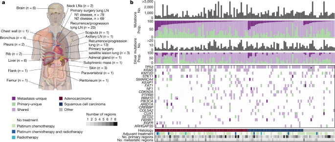
Presence or absence of driver mutations in cancer genes that contained a driver mutation in at least 10% of the cohort. The driver changes in CDKN2A, KEAP1, KMT2D, KRAS, SMARCA4,STK11 and TP53 were included.

Three separate relevant publications23,24,25 were identified for SETD2, only one for KDM5C83 and none for KMT2B. Therefore, we proceeded to focus solely on the impact of SETD2 on CN-independent ASE. This was done in lung cells (H1650; three biological replicates with shRNA knockdown23), kidney cells (786-0; single replicate with ZFN knockout24) and liver cells (HepG2; single replicate with CRISPR-mediated knockout25).

Because the libraries used for RNA-seq were stranded, variant reads from each strand were compared to obtain the difference in strandedness relative to the total depth at the variant position.

The ten editing events we selected were all done with the orthogonal method and included in the data table 2.

To test the potential relationship between signature activity and the expression of specific genes, we performed a linear mixed-effects model using the number of RNA variants attributed to each signature as the dependent variable, and gene expression of all genes in our dataset (n = 20,136). The log10 was calculated for genes with at least five read counts in 20% of the cohort.

A linear mixed-effects model was created to further compare the relationship between the expression of the genes and the tumour, using the number of RNA variants attributed to the tumours as the dependent variable.

APOBEC motif enrichment analyses were performed based on a previously reported local enrichment method93. In brief, for each C>T variant site, a Fisher’s test was performed to test whether C>T changes within 20 upstream or downstream nucleotides occurred more than expected by chance at specific motifs (CAT[C>T]) in either strand.

Source: https://www.nature.com/articles/s41586-023-05706-4

I-TED and the ITH of other forms of alterations: a multivariable linear regression study. Computational analysis and application to COSMIC mutational signatures

The relationship between I-TED and the ITH of other forms of alterations was tested using a multivariable linear regression in a similar fashion as that detailed in the section ‘I-TED’.

Clinical features, including age of the patient, sex, years spent smoking cigarettes and TNM stage of the primary tumour at resection. For more information on how these features were obtained, check out the methods in the companion manuscript.

LUAD-specific subtype as defined by central pathological review (acinar, lepidic, cribriform, micropapillary, mucinous, papillary or solid). This feature is described in a companion paper and was only available for LUAD tumours.

The number of expressed mutations is divided by the total amount of mutation in the tumours region. If the data contains at least three reads of a certain allgene, then the mutation is said to be expressed. This metric serves as a proxy for the proportion of tumour mutations that were present in the bulk RNA-seq transcripts.

Similarly, the number of events that occur in the same place was also taken into account. Details on how genome-doubling events per tumour region were calculated are available in a companion paper7.

COSMIC mutational signatures SBS1, SBS2, SBS4, SBS5, SBS13 and SBS92 (ref. 34). Signature activity was measured as the fraction of mutations per tumour region corresponding to each signature’s weight. The combined two signatures were used for the activity of the disease. The companion manuscript contains information about how the signatures were obtained.

To measure the impact of expression diversity within a tumour, we included the per tumour region I-TED score. I-TED was imputed as the median score across the cohort for samples for which only one region per tumour was available.

The three genes reported to play a role in cancer development from the literature are AZIN1,COPA and COG3. This feature was added only for tumour regions with at least 30 unique RNA reads covering the editing sites of interest.

Source: https://www.nature.com/articles/s41586-023-05706-4

A Structured Machine Learning Framework Using Tensorflow (v.2.6.0)104, sklearn(v.0.0)105

We built the machine-learning framework in Python using Tensorflow (v.2.6.0)104 and sklearn (v.0.0)105. Specifically, we built an ensemble classifier that used three different model types: (1) logistic regression, (2) random forest and (3) multilayer perceptron with support vector machine embedded in the final layer. The structure of the machine-learning pipeline is described here.

We took out the features with high correlation coefficients and examined the correlation structure among the potential explanatory features. We one-hot-encoded categorical features using get_dummies from Pandas (v1.3.3)106 and then split the data into training and test datasets (75/25 split). We had 60 features after we were done with decoding. We scaled the features with MinMaxScaler and SMOTENAc to improve the balance of the dataset. Finally, we used the sklearn (v.0.0)105 framework to perform additional variable selection before training using a LinearSVC model (penalty = “l1”), keeping those features with importance ≥0.015. This threshold removed 15 out of 60 features. Following this initial pre-processing, we generated different subsets of the dataset depending on the source of the input features, thus downstream processes within the pipeline operated on three datasets: (1) genomic only features, (2) transcriptomic only features, and (3) all features.

For each model type, to tune model hyperparameters, we performed a randomized grid search with RandomizedSearchCV (sklearn.model_selection, v.0.0)104 and StratifiedKFold cross-validation (n_splits = 10, n_iter = 500).

A categorical hinge loss function was used in the last layer as a way to cut overfitting and use a sequential model. The final layer of the sequential model constitutes a support vector machine using this approach. The Adam is an optimizer from tensorflow.keras.optimizers. We defined a search grid that would tune the following parameters: learning rate, batch size, amount of hidden layers, number of hidden layers and sizes of hidden layers. Following the cross-validated training across the randomized search grid, we selected the best performing model according to the greatest balanced accuracy. PermutationImportance from eli5.sklearn is how we extract feature weights from this model. To determine the performance of the selected model on held out test dataset, we used the model to predict whether or not a test region was seeding or not and compared this to the true labels. The machine-learning pipeline was developed using Python (v.3.5.5), and plots of results were generated in R (v.4.0.3) using ggplot2 (v.3.3.5).