Overconfidence in the climate

Assessing the UN Environment Programme Emissions Gap Report 2023: A Probabilistic Approach using a Simple Climate and Carbon Cycle Model FaIR v.1.6.2

The United Nations Environment Programme. Emissions Gap Report 2023: Broken Record – Temperatures Hit New Highs, yet World Fails to Cut Emissions (Again) (UNEP, 2023); available at https://go.nature.com/4ebr5ub.

If the world wants research and development of carbon-removal technologies, they need to stop pumping pollution into the atmosphere. The UK shut down its last coal-fired power plant on 30 September and announced investments of over 2 Billion dollars in carbon capture and storage technologies over the next 25 years. The projects will be situated in two of the country’s poorest coastal regions, bringing much-needed skilled jobs, training and research to areas that have been hit hard by deindustrialization. These efforts are a start.

To estimate eTCREup (equation (1)), we directly use the warming outcomes reported in the PROVIDE ensemble. The warming outcomes are evaluated using the simple climate and carbon cycle model FaIR v.1.6.2 (ref. 55) in a probabilistic setup with 2,237 ensemble members consistent with the uncertainty assessment of IPCC AR656. Each ensemble member has a specific parameter configuration that allows for the assessment of ensemble member-specific properties such as the climate metrics introduced above across different emission scenarios. This probabilistic setup of FaIR is consistent with the assessed ranges of equilibrium climate sensitivity, historical global average surface temperature and other important metrics assessed by IPCC AR6 WGI (ref. 18).

Estimating the effective Zero Emissions Commitment (eZEC) allows us to separate the stabilization and decline components of NNCE. We evaluate eZEC using the warming outcome of the original PROVIDE REN_NZCO2 scenario.

where n refers to the ensemble member from FaIR, t′ is the time step, Et′ is the net CO2 emissions in time step t′ and Tt′(n) refers to the warming in the time step t′ for a given ensemble member.

NNCE Simulations of the PROVIDE REN_NZCO2 Scenario with Diverse Levels of Carbon Emissions after the Year of the Paris Agreement

$${{\rm{NNCE}}}{{\rm{stabilization}}}(n)=0\quad {\rm{if}}\;{T}{2060}(n) < 1.5\quad {\rm{else}}\,\frac{{\rm{eZEC}}(n)}{{{\rm{eTCRE}}}_{{\rm{down}}}(n)}$$

Peak warming depends on eTCREup, and each member demonstrates a different level of warming. We calculate the cumulative NNCE to ensure that the cooling of the ocean will be 1.5 C by the year 2200.

The effective transient response to cumulative emissions (up), or eTCREup: this metric captures the expected warming for a given quantity of cumulative emissions until net-zero CO2.

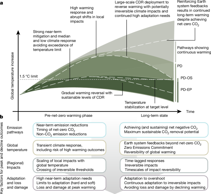
We analyzed the NNCE for the PROVIDE REN_NZCO2 scenario. The REN_NZCO2 scenario follows the emission trajectory of the Illustrative Mitigation Pathway (IMP) REN from the AR6 of IPCC52,53,54 until the year of net-zero CO2 (2060 for this scenario). After the year of net-zero CO2, emissions (of both GHGs and aerosol precursors) are kept constant.

Two sets of scenario ensemble were used to project the sea-level rise, permafrost and peatland carbon emissions. One of the scenarios achieved a net-zero GHG emission goal of the Paris Agreement and the other only achieved net- zero CO2 emissions, but both scenarios had a temperature rise of 2 C. Projections for sea-level rise are taken from the ref. 37, based on a combination of a reduced-complexity model of global mean temperature with a component-based simple sea-level model to evaluate the implications of different emission pathways on sea-level rise until 2300. For the scenario we use the permafrost module of the ESM OSCAR67 and a peatland emulator from the previously published peatland intercomparison project68. The data used to drive the modules is caused by GMST change and atmospheric CO2 concentration change. We used the CO2 and CH4 fluxes from both the north and south of the peatlands to make simulations. The net climate effects were computed using the method described in ref. There are 67. Taking into account the CH4 emissions is how we derive the CO2 warming-equivalent emissions.

Source: Overconfidence in climate overshoot

Modelling Regional Climate Differences: Averages between Peak Warming and Precipitation rates for SSP5-34-OS and SSP1-19

$${E}{{{\rm{CO}}}{2}\text{-}{\mathrm{we}}^{* }}={{\rm{GWP}}}{H}\times \left(r\times \frac{{\Delta E}{{{\rm{CH}}}{4}}}{\Delta t}\times H+s\times {E}{{{\rm{CH}}}_{4}}\right)$$

We smooth the GMST time series by applying a 31-year running average. Peak warming can be identified as the year in which this smoothed GMST reaches its maximum. Next, we select the years before and after peak warming in which the smoothed GMST is closest to −0.1 K and −0.2 K below peak warming. There is a model-dependent difference in the average time between the rate of change in GMST before and after peak warming. In each run, we average yearly temperatures and precipitation for the 31 years around the above-described years of interest. Finally, for each ESM, these 31-year periods are averaged over all available runs of the ESM and an ensemble median for the 12 ESMs is computed for the displayed differences.

We analyse the climate projections for the SSP5-34-OS and the SSP1-19 scenarios by using 12 of the 11 ecosmetry models in the project.

The average of the regional averages for land or ocean regions is computed by us. WNEU is comprised of land grids in western central Europe and northern Europe. The North Atlantic region above 45N has ocean grid cells. 3e,f). Land regions are AMZ and WAF.

We note that none of the two protocols includes land cover changes beyond the reference pathway. This points to an implicit assumption that the additional CDR in these simulations is achieved using technical options with little to no land footprint such as Direct Air Capture with CCS (Extended Data Table 2). If the amount of CDR was to be achieved using land-based CDR methods, however, we would expect pronounced biophysical climate effects from the land cover changes alone65. Regional climate differences should be explored in the future modelling efforts.

Governments and industry must have a laser-like focus on the risks ahead and how to mitigate them. This means aggressively cutting emissions in order to help communities cope with shocks. To scrub the atmosphere after it has been formed is to court disaster for the people and planet.

It’s not that carbon-removal methods don’t work. Some do. The simplest is, of course, planting trees. More-complex measures include extracting carbon directly from the atmosphere. But as Schleussner and his colleagues estimate, up to 400 gigatonnes of carbon would need to be removed from the atmosphere by 2100 to limit warming to 1.5 °C, assuming current emissions trajectories continue. In emissions terms, that is equivalent to running the US energy industry in reverse for around 80 years.