Predicting visual function with a wiring diagram

Analyses of the neurotransmitter predictions for LC10/LC15: I. Number of pathways, cell types, node shapes and type numerosities

The pathways begin at a hexel type, pass through an intermediary type, and then finish at a target type. The hexel type will not be used as the intermediary type. It is the cholinergic type that is restricted for LC10ev. For LC15, the constraint was unnecessary as the top intermediaries are all predicted to be cholinergic (excitatory). The analyses do not have to assign spatial locations for the intermediary types to be assigned. The number of cells for each intermediary type can be found in a companion paper4.

The number of cells of type B and the average number of scurvy received from A cells is two variables that can be normalized.

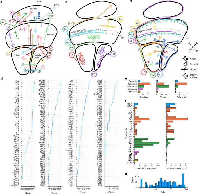
Nodes, representing cell types, are coloured by clusters. Node size encodes the number of drawn connections, so that types that are top input/output of many other types look larger. Node shapes encode type numerosities (number of cells of that type), from most numerous (hexagon) to least (ellipse) (see the figure legends). The lines show connections between cell types. The line colour encodes the relationship (top input or top output) and the line width is proportional to the number of synapses connecting the respective types. The neurotransmitter predictions are expressed by the line arrowheads.

An interpretation of the matrix Pab is as a random walk on a network of neurons. At each step, the walker chooses an input synapse of the present neuron at random, and crosses the synapse in the retrograde direction to get to the presynaptic node. Then Pab shows the chance of stepping from neuron b to neuron a.

Estimating the width of an ellipse on a hexagonal lattice and the length of a column using a single hexel

The closest neighbours are the next-nearest neighbours, which are constant away. Hexels were grouped with the same number of q or p. The resulting coordinate was in units of lattice constant (\times \sqrt{3}/2).

An ellipse approximation gives an estimate of the receptive field size. For a non-parametric estimate, I also used 1D projections onto directions defined on the hexagonal lattice. Each hexel was given coordinates (p, q), with the origin placed at the anchor location used for alignment.

(2sigma ) is defined as the width of a 1D Gaussian distribution for which the variance is. This is the full-width at ({e}^{-1/2}\approx 0.6) of the maximum. Alternatively, the width could be estimated by the full-width at half-maximum, (\sigma 2\sqrt{2\mathrm{ln}2}\approx 2.4\sigma ). The width is proportional to (sigma). I stick with the simplest estimate, which can be scaled by any factor of the reader’s preference.

The first term of the covariance matrix C effectively regards the probability distribution as a weighted combination of Dirac delta functions located at the lattice points. The second term is a correction that arises if each delta function is replaced by a uniform distribution over the corresponding hexagon. A column receives visual input from a non-zero solid angle. The length and width would disappear if there was a single hexel concentrated at a single Delta function. The length and width of an image that has a single non-zero hexel are affected by the correction. The correction becomes relatively minor when the length and width of the image are large.

in which I denotes the 2 × 2 identity matrix and s denotes the length of a hexagon side. The lengths and width of the hexel image are defined by (2sigma _max ) and (2sigma _min ). The ellipse is centered at the centroid, and oriented along the principal eigenvector.

Intrinsic cell types in the optic lobe of a flies I. Seeding and analysis of Drosophila2

The preprint was released to detail cell types in the adult male brain of a flies. The list of intrinsic cell types is almost identical to ours, apart from naming differences in new types. The results of the left and right eye parts of our female fly brain reconstruction match the ones analysed in the present paper. The brain replications of another individual fly and that of a same brain in another hemisphere provides additional validation of our findings.

Rules of connectivity in the optic lobe were simplified in a companion paper4 to depend on only cell type, and neglected spatial locations. The current work assigned hexel cell types to hexagonal lattices for a better characterization of the interdimensional landscape of the optic lobe.

Eventually morphology became insufficient for further progress. Expert annotators, for example, struggled to classify Tm5 cells into the three known types, not knowing that there would turn out to be six Tm5 types. At this point, we were forced to transition to connectomic cell typing. This could have been done much earlier. As mentioned above, connectomic cell typing must be seeded with an initial set of types, but the seeding did not have to be as thorough as it ended up. The challenge of extending the connectomic approach is something we have to worry about in the future.

Line amacrine cells were described in Strausfeld’s Golgi studies of Calliphora and Eristalis1, as well as Musca65. There are still unpublished observations of line amacrine cells. Line amacrine cells were named Dm3 in a Golgi study of Drosophila2.

Light microscopes with multicolour labelling3 went beyond Golgi studies by splitting Dm3 into two types with different orientations of dendrite. Dm3p and Dm3q have transcriptomes that differ before adulthood. The alternative names were Dm3a and Dm3b. Immunostaining showed that Dm3q expresses Bifid, whereas Dm3p does not. Ref. 18 also analysed a reconstruction of seven medulla columns64, with the results showing that Dm3p and Dm3q prefer to synapse onto each other, foreshadowing the present work, and speculatively placed Dm3 cells in the motion pathway.

TmY9 was previously described. The two TmY9 types can be distinguished by the tangential directions of their neurites (Fig. 2b,c), or by their connectivity (Fig. 3a, and Extended Data Figs. 4 and 5). The profiles of their groups are slightly different. Tm Y9q only covers the first layer of the lobula plate while TmY9q covers the second and third. TmY9q⟂ is more often bistratified in layers 5 and 6 of the lobula, whereas TmY9q is more often monostratified (Figs. 1a and 2b,c).

LC10 cells project from the lobula to the anterior optic tubercle12, and have been linked with visually guided courtship behaviours66. Four LC10 types were identified using GAL4 lines on the basis of their stratification in the lobula13. I was able to identify a fifth type by using the connectomic approach. LC10e was further divided into two groups based on their internet connection. The two groups cover the dorsal and ventral medulla, respectively.

It’s possible that the LC10e can detect a corner or T-junction in the ventral variant.

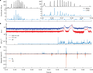
The neurotransmitter at each synapse was predicted directly from the EM images using a trained convolutional neural network with a per-synapse accuracy of 87% (refs. There are 3 quotes. The probability of a synapse to be one of the six primary neurotransmitters in Drosophila is calculated with the use of the algorithm. We then averaged these probabilities across all of a neuron’s outgoing synapses, under the assumption that each neuron expresses a single outgoing neurotransmitter, to obtain a 1 × 6 probability vector representing the odds that a given neuron expresses a given neurotransmitter. We then assigned the highest-probability neurotransmitter as the putative neurotransmitter for that neuron. The per-neuron accuracy is 94%. In cases in which the highest probability p1 < 0.2 and the difference between the top two probabilities p1− p2 < 0.1, we classified the neuron as having an uncertain neurotransmitter. In around 1,600 Kenyon cells, where the neurotransmitter is known to be ach, the neurotransmitter prediction could be seen as overwritten by the known neurotransmitter.

Whether a neurotransmitter has an excitatory or inhibitory effect on the postsynaptic neuron depends on the identity of the postsynaptic receptor. The brain of the fly can use Acetylcholine when the postsynaptic receptor is nicotinic. The postsynapticreceptor is in the center of the animal’s body.

On the use of hexagonal lattices for retinal imaging. I. Dm3 cells and connections in the v783 reconstruction

According to transcriptomic data19,68, Dm3 expresses GluClα. Unpublished data shows that both TmY4 and TmY9 express personal communication with Y.Kurmangaliyev. Dm3p and Dm3q have transcriptomic information, but not Dm3v.

The predictions for LPi14 and Lpi15 have been made on the basis of electron micrographs, which show that they are likely to be inhibitory. LPi07 cells are predicted to be GABAergic, glutamatergic or uncertain on the basis of electron micrographs, and are presumed to be inhibitory.

The hexagonal lattices are drawn to look exactly like the figures. The drawings are meant to show the nearest-neighbour relations of the cells and columns. More accurate representations of the lattices were constructed in ref. 29, which demonstrated how lattice properties vary in space for the left eye of many flies. Visual acuity also varies across the retina in flies and other insects52,77.

Tm1 is OFF transient30,32,72, Tm2 is OFF transient30,32,72,73, Mi4 is ON sustained30,74, Tm9 is OFF sustained30,32,72, and L3 is OFF sustained33,75. These are all Dm3 inputs (Extended Data Figs. 1 and 3), consistent with the prediction that Dm3 cells have OFF receptive fields. Mi1 is on. Calcium images are used in most of these studies. The possibility of electrophysiology and voltage imaging47 is also possible.

Connectivity maps included 745 Tm1, 746 Tm2, 716 Tm9, 796 Mi1, 749 Mi4, 730 Mi9, 785 L1, 763 L2, 709 L3, 671 L4 and 774 L5 cells in the v783 reconstruction that were successfully assigned to points in the hexagonal lattice through the procedures explained below. These numbers are smaller than the total number of cells proofread in v783 (ref. 4), but the deficit is generally less than 10%.

The Mi1 cells were automatically assigned to hexagonal lattice points. L cells were assigned locations based on where they were placed in one-to-one correspondence with Mi1 cells. The Hungarian Algorithm assigned the locations of other hexel types by placing them in one-to-one correspondence with L cells.

The resulting locations of hexel types in (p, q) coordinates are provided in Supplementary Data 2. All three axes of the hexagonal lattice point have been defined by the convention. The vertical axis is directed dorsally. The p and q axes are in the same location in the medulla. The lattice for the flies is oriented with points on both sides and flat sides at the top and bottom. The relation of p–q axes to dorsoventral and anteroposterior axes is more complex than indicated in Fig. 1f, because the medulla is curved rather than flat.

The figures show the lattice of medulla columns. A similar lattice can be constructed for ommatidia, and this lattice is left–right inverted relative to the lattice of medulla columns owing to the optic chiasm. It is shown by the motion on the medulla lattice and on the retina. In other words, the p and q axes are swapped in the eye relative to the medulla. Another difference between the eye and the medulla is that the p and q axes are close to orthogonal in the medulla, which is squashed along the anterior–posterior direction. The p and q axes are more similar to a hexagonal lattice, with the p and q axes roughly 120 apart in the eye.

Cell type assignments in a hexagonal lattice. Part II: The centroid coordinates and discriminator families of Pm cells

Suppose that an image has hexel values between 1 and N points in a hexagonal lattice. Normalizing the image yields a probability distribution ({p}{i}={h}{i}/({\sum }{j=1}^{N}{h}{j})). Then calculate the coordinates of the centroid.

The limits are found in the C.

We found that it was sufficient for feature dimensions to include only intrinsic types (T = 227). Alternatively, feature dimensions can be defined as including both intrinsic and boundary types (T > 700), and this yields similar results (data not shown).

The sums are similar to an equation. Normalizing by degree yields output fractions of type Wst/Ds+, wheret runs from 1 to T. The input fractions of type t are similar to those given by Wst/Dt.

On the basis of the auto-correction procedure, we estimate that our cell type assignments are between 98% and 99.9% accurate. Theradius is the average distance from its cells to its center, calculated as the quality of our cell typing. The calculation of the center was made using the total distances from each cell in the type to the centre. A large type radius is a sign that the type contains different types of cells. For our final types, the radii vary, but almost all lie below 0.6 (Extended Data Fig. 3b). Lat has an exceptionally high type radius, and deserves to be split (see the ‘Cross-neuropil tangential and amacrine’ section). If ornot boundary types are included in the feature Vector, the type radii are essentially the same.

Supplementary Data 4 contains discriminators for all types in all families. Many although not all discriminations are highly accurate. Both intrinsic and boundary types are included as discriminative features.

The Pm family can be visualized in two-dimensional space of the C3 input fraction and TmY3 output fraction. The Pm cells in this space can be discriminated against by the input fraction and TmY3 output fraction. This conjunction of two features is a more accurate discriminator than either feature by itself.

On the quality of predicates for sub-boundary types – a case study involving Jaccard’s Distance Algorithm

We also measured the drop in the quality of predicates if excluding boundary types (where the predicates are allowed to contain intrinsic types only). The weighted mean F-score is a small indicator of how marginal the impact on predicates is.

On a high level, the process for computing the predicates is exhaustive—for each type, we look for all possible combinations of input type tuples and output type tuples and compute their precision, recall and F-score. There are a few techniques that are used to speed up the computation like calculating minimum precision and recalling thresholds from the current best candidate.

Because the feature vector is rather high dimensional, it would be helpful to have simpler insights into what makes a type. One approach is to find a set of simple logical predicates based on connectivity that predict type membership with high accuracy. The attribute is connected to some cell of type t, and the attribute is connected to another cell of type t.

The number of positive predictions made by the logical predicate is the total of true positive predictions.

Once we arrived at a list of types, we used the trimmed mean to estimate the centre of each type. Then, for every cell, we computed the nearest type centre by Jaccard distance. The nearest type centre was found for 98% of the cells. We sampled some disagreements and reviewed them manually. In the majority of cases, the algorithm was correct, and the human annotators had made errors, usually of inattention. The remaining cases were mostly attributable to proofreading errors. There were also cases in which type centres had been contaminated by human-misassigned cells (see the ‘Morphological variation’ section), which in turn led to more misassignment by the algorithm. The automatic corrections were applied to all the cells that were rejected using distance thresholds.

For the hierarchical clustering of cell types (Fig. 2c), the feature vector for each cell type is obtained by concatenating the vectors of input and output fractions for that cell type.

Citizen scientists created farms in FlyWire or Neuroglancer with all the found cells of a given type visible. Farms showed visually where cells still remained to be found. If they found a small bald spot, it was a popular method to move the 2D plane in that place and add segments to the farm to look for cells of the correct type. Farms also helped with identifying cells near to the edges of neuropils, where neurons are usually deformed. It was possible to make a calculation about how a cell should look at the edge if there was a view of other cells of the same type.

Citizen scientists created a comprehensive guide with text and screenshots that expanded on the visual guide. Any publicly available scientific literature about the brain was also studied. They shared findings at discuss.flywire.ai, which as of 10 October 2023 had over 2,500 posts. Community managers shared findings from the scientific literature and gave feedback to citizen scientists.

Additional community resources (discussion board/forum, blog, shared Google drive, chat, dedicated email and Twitch livestream) fostered an environment for sharing ideas and information between community members (citizen scientists, community managers and researchers). Community managers answered questions, gave resources, and helped organize the community. Daily stats including number of annotations submitted per individual were shared on the discussion board/forum to provide project progress. There was live interaction, demonstrations and communal problem solving in the weekly video livestreams. The environment created by these resources enabled citizen scientists to organize their activities in a number of ways.

Source: Neuronal parts list and wiring diagram for a visual system

Connectomic Cells: Anatomy and Analyses of the Left and Right Brains from a Citizen Scientist’s View of the Cells

Citizen scientists were given a visual guide to the cells. FlyWire made available 3D meshes which indicate the four main brain areas. The visual identification was based on the cell structure. In the beginning it was suggested to label type families such as Dm, Tm, Mi and so on. Over time, the annotations of certain types developed. A software tool that enabled easy selection and submission of preformatted type names was used to enforce the use of canonical names.

The top 100 players from Eyewire79 had been invited to proofread in FlyWire24. They were encouraged to label neuron when they felt confident after 3 months of having their right brain checked. A majority of citizen scientists do a mixture of both. Sometimes they would look for cells of a specific type to make sure they didn’t miss anything.

Our connectomic cell approach to typing is initially seeded with some set of types, to define the feature vectors for cells (Fig. 2a), after which the types are refined by computational methods. The initial seeding was done with the use of a time-honoured approach of cell typing and computational tools. morphology is a misconception because it only refers to shape. The influence of orientation and position in the hierarchy of neural layers is more fundamental. Thus, ‘single-cell anatomy’ would be more accurate than morphology, although the latter is the standard term.

It is possible that a connection doesn’t exist from other studies. T1 cells lack output. Therefore, in our analyses, we typically regarded the few outgoing T1 synapses in our data as false positives and discarded them.

The matrix needs to be looked for extreme asymmetry. If there is a larger number of synapses from A to B, then the connection may be spurious. The large contact area between A and B means more chances of false-positive synapses from B to A.

The mirror twin in the opposite hemisphere is what differentiates the cell types in the central brain. The cardinality in the hemibrain is cut to one. Therefore, whether there is a connection between cell type A and cell type B must be decided based on only two or three examples of the ordered pair (A, B) in all the connectomic data that is so far available. The threshold should be set to a relatively high value, in order for false positives to be avoided.

The seven column reconstruction28 provided a matrix of connections between their modular types. This shows good agreement with our data (Methods and Extended Data Fig. 9), providing a check on the accuracy of our reconstruction in the optic lobe. This validation complements the estimates of reconstruction accuracy in the central brain that are provided in the flagship paper24.

They are not modular because Tm21, Dm2, TmY5a, Tm 27 and Mi15 are less numerous than 800. On the other hand, some of our types (T2a, Tm3, T4c and T3) contain more than 800 proofread cells (Fig. 1d), which violates the definition of modularity. This partially agrees with the seven column reconstruction28, which regarded T3 and T2a as modular, and T4 and Tm3 as not modular. T4c is an unusual case as the other T4 types are below 800. It should be noted that all of the above cell numbers could still creep upward with further proofreading.

The cost function of Jaccard distance for the neuronal parts list and wiring diagram for a visual system (NEUROLOGY SYSTEM)

Optic lobe intrinsic neurons are almost entirely contained in one of the optic lobes (left or right), more precisely, 95% or more of their synapses are assigned to the five optic lobe regions listed above.

The inner and outer levels of the Flywire connectome are filled with 3,400 and 650 cells, respectively. These numbers are not inconsistent with modularity because photoreceptors are especially challenging to proofread in this dataset and under-recovery is higher than typical.

$$J\left({\bf{x}},{\bf{y}}\right)=\frac{{\sum }{t}\min \left({x}{t},{y}{t}\right)}{{\sum }{{t}^{{\prime} }}\max \left({x}{{t}^{{\prime} }},{y}{{t}^{{\prime} }}\right)}$$

The weighted Jaccard distance d(x,y) is defined as one minus the weighted Jaccard similarity. The quantities are always between zero and one. In our cell typing efforts, we have found empirically that Jaccard similarity works better than cosine similarity when feature vectors are sparse.

This cost function is convex, as d is a metric satisfying the triangle inequality. Therefore, the cost function has a unique minimum. We used various approximate methods to minimize the cost function.

Source: Neuronal parts list and wiring diagram for a visual system

Diagrammatic Study of Type Mixing in a Neuronal Parts List and Diagram for a Visual System from Cytoscape 81

For auto-correction of type assignments, we used the element-wise trimmed mean. We found empirically that this gave good robustness to noise from false synapse detections. The coordinate descent approach was used to minimize the cost function with respect to each ci. The loop did not include the i for which ix was non-zero. This converged within a few iterations of the loop.

The types in each cluster are usually from multiple families. Sceptics might regard such mixing as arising from the ‘noisiness’ in the clustering noted above at the largest distances. The closest types to the center tend to be from the same family. There are lots of mergers between different families at intermediate distances. Thus, some of the mixing of types from different neuropil families seems genuinely rooted in biology.

The wiring diagrams were drawn with the help of Cytoscape 81. Organic layout was used for Figs. 3 and 7c, and hierarchical layout was used for the others. The layout tries to make the arrow point downward. After Cytoscape automatically generated a diagram, nodes were manually shifted by small displacements to minimize the number of obstructions.

Source: Neuronal parts list and wiring diagram for a visual system

Boundary Neurons (Class, Family and Type): Axons and Carcinones Over the Dorsal Amacrin

Boundary neuron are those that have at least 5% of their cells in the optic hemisphere, and can either project or shoot images.

In the main text (in the ‘Class, family and type’ section), we used the term ‘axon’. An axon is defined as some portion of the neuron with a high ratio of presynapses to postsynapses. This ratio could be high in a way. The axon might have a very high ratio compared to the dendrite. In either case, the axon is typically not a pure output element, but has some postsynapses as well as presynapses. For many types it is obvious whether there is an axon, but for a few types we have made judgement calls. The presence of presynaptic boutons can sometimes be used to recognize the axon. The opposite of an axon is a dendrite, which has a high ratio of postsynapses to presynapses.

There are four different types of amacrines over the medulla and lobula. T2a and T3 are connected to T4 and T5 by the link of LMA1 to LMA4. The LMa family could be said to include CT1, a known amacrine cell that also extends over both the lobula and medulla. However, the new LMa types consist of smaller cells that each cover a fraction of the visual field, whereas CT1 is a wide-field cell.

The DRA differs from the rest of the retina in its organization of inner photoreceptors. The output cell types in non-DRA and DRA are different. Specifically, DRA-R7 connects with DmDRA1, whereas DRA-R8 connects to DmDRA254,87. These distinctive connectivity patterns result in DmDRA1 and DmDRA2 types exhibiting an arched coverage primarily in the M6 layer of the dorsal medulla (Fig. 9b). R7-DRA and R8-DRA are incompletely annotated at present, and this will be rectified in a future release. DmDRA1 receives R7 input, but sits squarely in M7. We did not change the name because of historical reasons, but this could be seen as an Sm type.

A Tlp neuron is going from plate to plate. Tlp11 to Tlp14 was defined later on 10. We have identified five of them. Tlp11, TLP12 and Tlp13 need to be retired10, as these types can be identified with Tlp5 and TLP1, respectively.

Pm1, 1a and 26 were each split into two types. Pm3 and 4 are the same as before. In order to increase cell volume we identified six new Pm types, numbered Pm01) to Pm14, for a total of 14 Pm types. The new names can be distinguished from the old ones by their zeros. All are projected to be giaergic. Pm1 was split into Pm06 and Pm04, Pm1a into Pm02 and Pm01, and Pm2 into Pm03 and Pm08.

Source: Neuronal parts list and wiring diagram for a visual system

LPi1-LLPt: A type of tangential neuron that projections from the lobula to the plate: Correspondences with old naming systems

We discovered one tangential type that projected from the lobula to lobula plate, and called it LLPt. This is a single type, not a family.

Now that LPi types have multiplied, stratification is no longer sufficient for naming. The naming system could be salvaged by adding letters to distinguish between cells of different sizes. For example, LPi15 and LPi05 could be called LPi2-1f and LPi2-1s, where ‘f’ means full-field and ‘s’ means small. To increase the average cell volume we chose the nameLPi05 toLPi15. Correspondences with old stratification-based names are detailed in Codex.

When identifying large recurrent neuropil-specific neurons (Fig. 5g) we applied the following criteria. The neurons were in the right place and met the criteria. The sub network of a single neuropil was at least half of the neuron’s incoming connections. At least 50% of the outgoing connections are contained within the same neuropil.

If Dm8 cells express DIP, they are divided into two types: yDm8 and pDm8. Physiological studies demonstrated that yDm8 and pDm8 have differing spectral sensitivities89. The main dendrites of yDm8 and pDm8 were found to connect with R7 in yellow and pale columns, respectively. On the basis of its strong coupling with Tm5a, our Dm8a probably has some correspondence with yDm8, which is likewise selectively connected with Tm5a51,53. It is not yet clear whether there is a true one-to-one correspondence of yDm8 and pDm8 with Dm8a and Dm8b. Dm8a and Dm8b prefer to go onto Tm5a and Tm5b together. Tm5a and Tm5b are not in correspondence with yellow and pale columns. The main branch of Tm5a is in yellow columns, while the other branches are in pale columns. Dm8a and Dm8b cells are roughly equal in number, the yDm8:pDm8 ratio is likely to be more than one51,53, similar to the ratio of yellow to pale columns. Thus, the correspondence of Dm8a and Dm8b with yDm8 and pDm8 is still speculative. When accurate photoreceptors become available, the yellow/pale issue should be reexamined.

Clustering metrics across the whole-brain and within-region (neuropil) neuronal subnetworks of a single neuron

All cells can be reached through directed pathways through the subnetworks of sccs. The directionality of connections is ignored when choosing a criterion called a WCC.

For a given neuron i, the in-degree ({d}{i}^{+}) is the number of incoming synaptic partners the neuron has and the out-degree ({d}{i}^{-}) is the number of outgoing synaptic partners the neuron has. The sum of in-degree and out-degree is termed the total degree of a neuron.

Our model has two zones of probability, a close one and a distant one, which are influenced by the distribution of connection probability. The data was extended in the data fig. 1e The probabilities in these two zones were derived from the real network. Then, for every neuron pair (around 14 billion pairs), we generate a random number drawn uniformly from between 0 and 1. The distance between the two neuronal arbours sets the probability of forming an edge between the pairs, pclose or pdistant. The connection between these two neurons is formed if the random number is below the threshold.

The global clustering coefficients is based on a supposition that for three of the same neurons, and, they are connected.

We computed these metrics both across the whole-brain and within-brain-region (neuropil) subnetworks. We counted all three-node motifs in our analysis, and made sure that no duplicate ones would be found, as well as the existence of distinct directed three-nodes. The expected prevalence of the specific neurotransmitter motifs was calculated under the assumption that neurons connect independently of neurotransmitter. We then compared this expectation to the true frequency of motifs with these neurotransmitter combinations.

We adopted a generalized ER model because the expected number of reciprocal edges were overstated in the wiring diagram. The generalized ER model ({\mathcal{G}}(V,{p}^{{\rm{uni}}},{p}^{{\rm{bi}}})) has two parameters, unidirectional connection probability puni and bidirectional connection probability pbi, both of which are set to match the wiring diagram. We had defined the sets of edges as:

Source: Network statistics of the whole-brain connectome of Drosophila

Directed configuration model for whole-brain connectome of Drosophila with preserving degree sequences and spatial densities from internal connections

$$\begin{array}{c}{E}^{{\rm{uni}}}\,:= \,{(i,j){\rm{| }}(i,j)\in E\wedge (j,i)\notin E},\ {E}^{{\rm{bi}}}\,:= \,{(i,j){\rm{| }}(i,j)\in E\wedge J,i, is E.endarray.

Pleft[i_ nrightarrow,j right] was counted.

The directed configuration model was used with consistency and preserves degree Sequences. We randomly select two edges in each graph and switch their endpoints under the switch-and- hold mechanism, to sample 1,000 random graphs that were uniformly from a configuration space of graphs. With these conditions, this CFG model is mathematically equivalent to the Maslov–Sneppen edge-swapping null model66,67,68.

To provide a more tractable spatial null model while preserving degree sequences, we developed the NPC model. This model has a degree-corrected block model. Each neuron was assigned to one of the 78 blocks based on which one had the most outgoing sachs. During random rewiring, the inter- and intra-neuropil connection probabilities are preserved. Moreover, like in the CFG model, we keep the degree sequences unchanged during randomization and prohibit self-loops and multiple edges. The interneuropil connection densities implicitly contain mesoscale spatial information. These constraints also mean that the total number of internal edges in each neuropil remains the same after reshuffling.

One can tie the 0–1 adjacency matrix (Ain mathbbR_ge 0nTimes n) to a strongly connected graph G (V,E) and a connection from neuron i to neuron j.

Source: Network statistics of the whole-brain connectome of Drosophila

The $alpha$-pinning state in Drosophila is a nonlinear whole-brain system: $mathcalL=12left(Pi frac

$${\mathcal{L}}=I-\frac{1}{2}\left({\Pi }^{\frac{1}{2}}{P}_{\alpha }{\Pi }^{-\frac{1}{2}}+{\Pi }^{-\frac{1}{2}}{P}^{\top }{\Pi }^{\frac{1}{2}}\right),$$

Source: Network statistics of the whole-brain connectome of Drosophila

The rich-club neural network: A three way model and its application to the whole-brain ER graph and integrator networks of the whole brain

We did a three way calculation of the rich club coefficient by sweeping by total degree, in degree and out degree. When the total degrees of the remaining nodes surpass 37, the network becomes denser compared with randomized networks. The peak occurs at total degree = 75. The model predicted that 38.7% of the cells would have a degree of 75. Once the minimal total degree reaches 93, the network becomes as sparse as the randomized counterpart. We considered rich-club neurons to be a subnetwork because they exhibit denser interconnections. In terms of degree, the range is between 10 and 54. Considering out-degree alone did not reveal any specific onset or offset threshold for rich-club behaviour, as the subnetwork always remains sparser than random. The NPC model has a rich-club coefficients. The null model was computed similarly with 100 samples.

The standard method of determining the rich-club threshold is to look for values of k for which Φnorm(d) > 1 + nσ, where σ is the s.d. of ΦCFG(d) and n is chosen arbitrarily20. However, as the s.d. from our samples is extremely small (approaches 0) near the bump in relative rich-club coefficient, we chose instead to define the onset threshold of the rich club as Φnorm(d) > 1.01 (1% denser than the CFG random networks).

The connectome is quantified by comparing it to an ER graph. The average undirected path length in the ER graph, denoted as ({{\ell }}{{\rm{rand}}}), is estimated to be 3.57 hops, similar to the observed average path length in the fly brain’s WCC (({{\ell }}{{\rm{obs}}}=3.91)). The ER graph’s clustering coefficients is small, much smaller than the observed ones. (Table 2). The whole-brain fly connectome is smaller than the world.

Similarly, we identified integrator neurons by filtering the intrinsic rich-club neurons for those that had an in-degree that was at least five times higher than their out-degree:

We used different subsets of sensory neurons as seeds in the model. We also ran the model using the set of all of the input neurons as seed neurons. The rank of the brain’s neurons was normalized and they were ranked by their distances from each other. We rank the visual projectionocytes as a proxy for visual sensory inputs to the central brain, but note that this is not a true sensory population.