Carbon was released through modern rivers
Hydro ATLAS: A forest model to study potential drivers of river DIC, CO2 and CH4 in the Peking University AMS facility
We used the hydro ATLAS information and a forest model to explore the potential drivers of the F14C content of river DIC, CO2 and CH4. The model was run separately for the 10 km 2 and 10 km 2 areas to make sure that they did not have any issues with the model.
Samples collected in 2017 and 2018 were processed and analysed at the Peking University AMS facility (PKU_AMS) in Beijing, China, following ref. 59. The water samples were acidified and shaken and heated to 75C to convert DIC to CO2. The CO2 was then purified cryogenically on a vacuum line and graphitized using zinc reduction. The samples collected in 2023 were analysed at a facility in Florida. Acidified samples were taken out of the water with N2 or Ar gas bubbling through them. The resulting CO2 was collected cryogenically and graphitized using hydrogen reduction of the CO2 sample over a cobalt catalyst. Internal testing samples and the background were processed alongside the samples in the PKU andBeta labs.
A multiclass classification of hydroatlas biome and the size of the river Xeric-Norden (Yukawa)
The information we got about the size of the river made for two classifications. (1) A binary ‘small’ (≤10 km2) and ‘large’ (>10 km2) classification—this classification was chosen owing to the lower river basin size limit of the HydroATLAS (10 km2) and was based on the exact/estimated catchment size information extracted from the original studies. This binary size class was used primarily for QA/QC checks in the database and also in defining whether to use reach or catchment parameters from HydroATLAS in the random forest model (Extended Data Figs. 3 and 4). A multiclass exponential classification of 0 to 100,000 km2, 10,000 to 100,000 km2, and one million to 100,000 km2 were used. The size classifications are provided in Supplementary Table 1.
Deserts, which included HydroATLAS biome ‘13. Deserts & Xeric Shrublands’ and also a further classification ‘15. There are samples from the polar desert in the database.
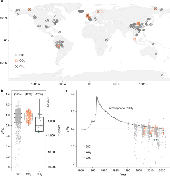
The F14C values were normalized in the database for each measurement in order to have a better representation of the F14C content in the atmosphere.
Some locations were looked at more than once. This is because of a combination of experimental approaches, for example, repeat sampling, exploration of temporal variations and method development. We took the average of the F14C observations at that location and made a new radiocarbon age and uncertainty 61 by repeating the sample location more than four times. The total number of observations was 1,020 in theExtended Data Table 1.
Source: Old carbon routed from land to the atmosphere by global river systems
Measurement of Sedimentary Effects in China’s Mekong River and Taiwanese Rivers Using a Rotating Niskin Sampler
River water DIC samples from Taiwanese rivers and the Mekong River in Cambodia were collected using the methods outlined in refs. 18,58. In Taiwanese rivers, 1-l sampling bottles were submerged into the middle of the channel using a weighted Teflon sampler. On the Mekong River, near-surface samples were collected using a horizontally mounted Niskin-type sampler. The river water was then pumped into preweighed 1-l foil bags (FlexFoil Plus) and then filters were used to avoid any atmospheric air mixing. The bag was filled with water from a river and squeezed before closing so that no air was trapped. After the filled bag was weighed and stored at 4 C, it was shipped to the UK where it was frozen for about a week.
Sedimentary, which included the HydroATLAS classes ‘1. Unconsolidated Sediments (SU)’, ‘3. Siliciclastic Sedimentary Rocks (SS)’, ‘5. There are two types of rocks, the Mixed Formation Rocks (SM) and the Mixed Formation Rocks 6. Carbonate Sedimentary Rocks (SC)’.
One data point returned ‘No Data (ND)’ from the HydroATLAS lithology classes and was excluded from the lithology analysis. Data from Antarctica were also excluded from the analysis owing to a lack of lithology data (returning ‘Ice and Glaciers (IG)’ from the HydroATLAS lithology classes).
Source: Old carbon routed from land to the atmosphere by global river systems
A random forest model applied to the age of hydroatLAS data based on the F14Catm data and its application to the HydroATLAS Data Baseline
Statistical analyses were carried out in R version 4.1.1 (ref. 63). We used nonparametric Kruskal–Wallis tests with the kruskal.test function in R, supplemented by post hoc analyses consisting of Conover–Iman tests using the conover.test function and unpaired two-sample Wilcoxon tests using the wilcox.test function. We undertook linear regression analyses using the lm function. The figures depict the details of where each analysis is applied.
A random forest model was used to look at potential drivers of the age of river carbon emissions. A machine learning model called Random Forests integrate Regression trees to make predictions. This approach has proved to be successful in many environmental studies due to its capacity to capture and reconcile the interplay among variables. In this study, we use random forest models to investigate the relationships between key catchment characteristics extracted from HydroATLAS and F14Catm values in the database. We wanted to identify which variables had the strongest control on the river carbon emissions.
To avoid the results being influenced by correlated input variables, we first removed variables that correlated with other potential input variables because of a Spearman correlation greater than 0.6. The year of sample collection is shown in Supplementary Table 5.
We split the model into runs based on the reach of the rivers and the total amount of water in them. Owing to limits on the number of data points, we only applied the model to DIC data, in which observations were n > 100 when separated by size.
Source: Old carbon routed from land to the atmosphere by global river systems
Global analysis of the relationship between predictor variables and F14 Catm from partial dependence plots in the random forest model. I: river DIC and CO2
We looked at the relationship between predictor variables and F14 Catm with partial dependence plots. The partial dependence plots show how F14Catm changes when a given input variable (Supplementary Table 5) varies but all other variables are held constant in the random forest model. We performed the partial dependence analysis ten times (mirroring the ten iterations of random forest models from using tenfold cross-validation) and plotted the mean values from these ten runs, with the variability across the runs indicated by the shaded area (Extended Data Figs. 3 and 4).
In an ideal world, it would be possible to account for petrogenic inputs to DIC and CO2 for each watershed in the database (and potentially for each sampling point). To do this, we would need to use dissolved cation (Na+, Ca2+, Mg2+, K+) and anion (Cl−, SO42+, Re) data to assess the weathering acids and contributions from carbonate and rock organic matter weathering18,38,39. Most of the studies that report riverDIC and CO2 F14C results do not report dissolved ion data, and if they do they don’t report the necessary range of cation and anion measurements. As such, we take a global view using our mean F14C DIC values and assess the petrogenic inputs using global estimates of carbonate and rock organic carbon weathering rates.
$${\rm{Total\; river\; DIC\; flux}}\times {F}^{14}{{\rm{C}}}{{\rm{river}}}=({\rm{lateral\; DIC\; export\; to\; ocean}}+{{\rm{vertical\; CO}}}{2}\,{\rm{emissions\; flux}})\times (a\times {F}^{14}{{\rm{C}}}{{\rm{decadal}}}+b\times {F}^{14}{{\rm{C}}}{{\rm{millennial}}}+c\times {F}^{14}{{\rm{C}}}_{{\rm{petro}}})$$
A times of F 14rmC_rmdecadal.
We can then calculate the non-petrogenic F14C value (F14Cdecadal+millennial), because the petrogenic source is assumed to contain no radiocarbon (that is, F14C = 0.0). This provided an estimate of the F14Cdecadal+millennial = 0.978 to 1.007.
We couldn’t collect sitespecific concentration or emission flux data because of the lack of data from the F14C data. This means that we were not able to scale the F14C values in the database with local and regional emission fluxes (Supplementary Information section 4).