Data shows a lifetime of extreme heat for children
Geometric Analyses of Human Exposure to Global Climate Extreme Events and Population Size Estimation Using Population and Life Expectancy Data
We then quantify the human exposure to the extreme events in a way that facilitates comparison and aggregation. We consider all people in a grid cell exposed to a climate extreme in a particular year if the climate extreme occurs in that year. If this river flood or wildfire happens within a grid cell with a 0 0 grid, we assume that the person located in that cell would be affected by the event. We use demographic data to convert the annual exposure of humans to their lifetime exposure of births by summing up the individual event categories.
Estimating lifetime exposure to extreme events requires crossing life expectancy data at the country level with grid-scale exposure projections. Exposures are summed at the grid scale for each lifetime of every GMT trajectory, birth year, and country. This assumes life expectancy to be spatially homogeneous across each country. Exposure during the death years is also included in this sum by multiplying these exposure projections by the fraction of the final year lived. The maps can be used for country-wide exposure for each trajectory and year of birth.
To downscale this demographic information to the grid scale, we assume spatially homogeneous cohort representation and life expectancy. Birth cohort size is represented as the number of people of age 0 of a given birth year in a given grid cell. This is estimated by multiplying the absolute population of the birth year (using the annual grid-scale population totals from ISIMIP) by the relative size of the age 0 cohort (using the interpolated 0- to 100-year-old population totals from the Wittgenstein Centre cohort data). This study ignores age structure and life expectancy within a country.
The Inter-Sectoral Impact Model Intercomparison Project (ISIMIP2b) project: Exposures of grid-level sectors to extreme events and related indicators of vulnerability
Climate change impacts can be projected across sectors, such as agriculture, lakes, water and fisheries, with the help of the Inter-Sectoral Impact Model Intercomparison Project. The impact models that are used in ISimip2b are from a consistent set of bias-adjusted global climate models from phase 5 of the CMP5 that have been selected based on their availability of daily data. Impact simulations are run for pre-industrial control (286 ppm CO2; 1666–2099), historical (1861–2005) and future (2006–2099) periods. The RCPs 2.6, 6.0 and 8.1 of the GCM input dataset are used for future simulations. The annual, grid-scale fractions of exposure to each extreme event are calculated from impact simulations and input data. For the full details of these computations, we refer to ref. 12, but we summarize extreme event definitions below.
We use two grid-scale indicators of vulnerability to compare with our estimates of ULE to heat waves. The first is an ISIMIP2b GDP input dataset using concatenated historical and SSP2 time series covering 1860–2099 annually17. This dataset was disaggregated from the country to grid level using spatial and socioeconomic interactions among cities, land cover and road network information and SSP-prescribed estimates of rural and urban expansion46. The second indicator is the Global Gridded Relative Deprivation Index v.1 (GRDI; ref. 16), which communicates relative levels of multidimensional deprivation and poverty (0–100, least to most deprived). This deprivation score was created using six input components. First is the child dependency ratio, which is the ratio between the population of children and the working-age population (15–64 years). This can indicate vulnerability, for which high ratios indicate a dependency of supposed consumers and non-producers on the working-age (producing) population47. Second, infant mortality rates (IMR), taken as the deaths in children younger than 1 year of age per 1,000 live births annually, are a signal of population health and form a long-term Sustainable Development Goal of the United Nations48. Third, the Subnational Human Development Index (SHDI), an assessment of human well-being across education, health and standard of living, originates from the Human Development Index, the latter of which is considered one of the most popular indices to assess country-level well-being. The SHDI improves on the HDI in terms of spatial scale and in representing 161 countries across all world regions and development levels49. As rural populations are prone tomultidimensional poverty, low values in the ratio of built-up to non-built-up area signal high deprivation. The 5th and sixth components use the mean and slope of nighttime light intensity to indicate deprivation in areas of low nighttime light intensity. These input components range from 30 arc seconds (roughly 1 km) resolution to subnational regions and are harmonized in an ArcGIS Fishnet feature class for aggregation onto a 0–100 range representing low to high deprivation. For the final aggregation, the IMR and SHDI components are given half the weight of the rest of the inputs, given their coarser resolution. Generations face deprivation and vulnerability to climate extremes through the multiple dimensions of the GRDI. Our approach does not explicitly account for the adaptation to climate change, but our multidimensional approach provides relevant information on the current adaptation potential of local populations.
The findings, published in Nature on 7 May1, highlight the disproportionate burden that climate change places on today’s young people — and the need to limit global warming to safeguard future generations.
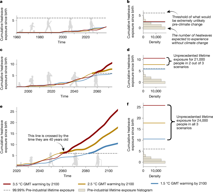
As an example, people who were born in 1960 and spend their lives in Brussels are projected to experience three heatwaves in their lifetimes. The average number of heatwaves for those born in 2020 will be 11, if warming can be kept to 1.5 C by the year 2200. If the temperatures reach 2.5 C and 3.5 C of warming, then that same group is projected to live through 18 heatwaves. (If all existing climate policies are implemented, global temperatures are expected to be 2.7 °C higher than in pre-industrial times by 2100.)
The researchers define this as a threshold of lifetime exposure to extreme weather that someone living in a world without climate change would have only a one in 10,000 chance of experiencing. Thiery says that climate change would make it impossible to experience many Climate Extremes if you are beyond that limit.
They used the demographic data to figure out how many generations would reach the limit across their lifetimes and how that would vary depending on different global-warming scenarios.