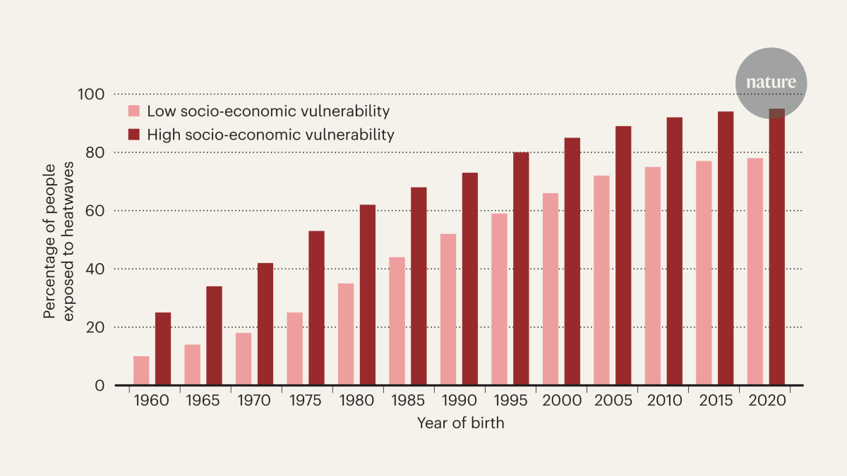
Climate risk is set to soar among younger generations

Exposure of Grid Cells to Extreme Heat Events, Tropical Storms, and Flood Hazards: Application to the AR6 Scenario Explorer

For heatwaves and disasters, we use pre-industrial thresholds to determine event occurrences, whereas for tropical storms, we use a single absolute threshold. Heatwaves affect an entire grid cell if the Heat Wave Magnitude Index daily (HWMId; refs. 34,35) of that year exceeds a threshold in the pre-industrial control HWMId distribution in that grid cell11. Although we refer to heatwaves throughout the paper, our definition refers to a 3-day extreme heat event that is expected on average once per century under pre-industrial climate conditions. Extreme heat events occur worldwide, but with different associated absolute temperature values. There are large intergenerational inequalities in lifetime heatwave exposure according to previous analysis. When crop yield falls below a threshold of their pre-industrial reference yield, the area occupied in a grid cell is used as the basis for crop failures. For 7 months, monthly soil water levels have to go above the pre-industrial level in order for a grid cell to be affected. The flooded area is the result of comparing daily discharge simulations from models of the global water sector to pre-industrial discharge. CaMA-Flood is used to convert discharge values to flooded areas. If a grid cell can sustain winds of 64 knots or more at least once a year, tropical storms can occur. Flood hazard associated with tropical cyclones don’t encompass exposure to tropical storms. When a grid cell is utilized to model a burnt area, there will be fires. If a model predicts burnt area sub-annually, it can be either the annual sum of monthly burnt area in case of an impact or capped at 100% of a grid cell. We reiterate that all exposure definitions here neglect potential exposure reduction measures and non-local effects.

A series of warming pathways are constructed and projected by the year 2031 based on the models used in the scenario explorer. The time series from the AR6 scenario explorer was chosen as the anchor point to produce the range of plausible time series. They were selected to reduce overshooting in the early years of low and higher GMT pathways, which can skew lifetime exposure estimates for early birth cohort. The upper bound was limited to 3.5 C in favour of more simulations, which is discussed further below. The choice of 1.5 C for the lower bound is more realistic than 1.0 C. The 1.5 C anchor scenario maximally reaches 1.57 C by the end of the century. It is referred to as 1.5 C throughout the analysis. The warming levels are reported compared to the pre-industrial temperatures. This yields a total of 21 GMT pathways for which we project CF.

We assume that life expectancy and cohort representation are variables that can be scaled to the grid scale. Birth cohort size is the size of the group of people who were born in a given year. This is estimated by multiplying the absolute population of the birth year (using the annual grid-scale population totals from ISIMIP) by the relative size of the age 0 cohort (using the interpolated 0- to 100-year-old population totals from the Wittgenstein Centre cohort data). Spatial variability in age structure and life expectancy within a country is therefore ignored in this study.

ISMIP2b: An inter-sectoral model intercomparison project to compare climate models vulnerability to heat waves and ULE

The Inter Sectoral Impact Model Intercomparison Project provides a simulation protocol for projecting the impacts of climate change across sectors. In ISIMIP2b, impact models representing these sectors are run using atmospheric boundary conditions from a consistent set of bias-adjusted global climate models (GCMs) from phase 5 of the Coupled Model Intercomparison Project (CMIP5) that were selected based on their availability of daily data and ability to represent a range of climate sensitivities17; the Geophysical Fluid Dynamics Laboratory Earth System Model (GFDL-ESM2M; ref. 30), the earth system configuration of the Hadley Centre Global Environmental Model (HadGEM2-ES; ref. 31), the general circulation model from the Institut Pierre-Simon Laplace Coupled Model (IPSL-CM5A-LR; ref. 32) and the Model for Interdisciplinary Research on Climate (MIROC5; ref. 33). Impact simulations are run for pre-industrial control (286 ppm CO2; 1666–2099), historical (1861–2005) and future (2006–2099) periods. Future simulations are based on Representative Concentration Pathways (RCPs) 2.6, 6.0 and 8.5 of GCM input datasets. Global projections of annual, grid-scale fractions of exposure to each extreme event category are calculated from ISIMIP2b impact simulations and GCM input data. For the full details of these computations, we refer to ref. 12.

We compare the vulnerability indicators to the estimates of ULE to heat waves. The first is a GDP input dataset using historical and SSP2 time series. This dataset was disaggregated from the country to grid level using spatial and socioeconomic interactions among cities, land cover and road network information and SSP-prescribed estimates of rural and urban expansion46. The second indicator is the Global Gridded Relative Deprivation Index v.1 (GRDI; ref. 16), which communicates relative levels of multidimensional deprivation and poverty (0–100, least to most deprived). The deprivation score uses six input components. First is the child dependency ratio, which is the ratio between the population of children and the working-age population (15–64 years). This can indicate vulnerability, for which high ratios indicate a dependency of supposed consumers and non-producers on the working-age (producing) population47. The infant mortality rate, taken as the deaths in children younger than 1 year of age per 1,000 live births annually, is a signal of population health and form a long-term goal of the United Nations. Third, the Subnational Human Development Index (SHDI), an assessment of human well-being across education, health and standard of living, originates from the Human Development Index, the latter of which is considered one of the most popular indices to assess country-level well-being. The SHDI improves on the HDI in terms of spatial scale and in representing 161 countries across all world regions and development levels49. Fourth, as rural populations are generally prone to multidimensional poverty50, low values in the ratio of built-up to non-built-up area (BUILT) signal high deprivation. The mean and slope are used to indicate the deprivation of areas with low nighttime light intensity. These input components range from 30 arc seconds (roughly 1 km) resolution to subnational regions and are harmonized in an ArcGIS Fishnet feature class for aggregation onto a 0–100 range representing low to high deprivation. The IMR and SHDI components are given less weight than the rest of the inputs, for the final aggregation. Generations face deprivation and vulnerability to climate extremes because of the multiple dimensions of the GRDI. Although our approach does not explicitly account for actual or potential adaptation to climate change, this multidimensional approach to vulnerability provides relevant information on the current adaptation potential of local populations.