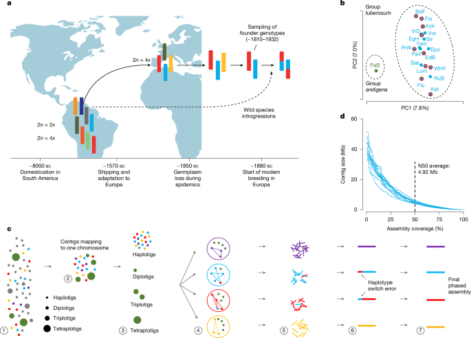
The pan-genome of a potato

Mapping and cloning of rice genome assemblies using InterProScan85 and BRAKER (v.1.6.0) in mapping-based mode

For functional annotation of genes, InterProScan85 (v.5.56-89.0) was used to predict potential protein domains. The first low quality read to be removed was used to calculate gene-expression levels. Then, the filtered paired-end reads were mapped against the index of decoy sequences, which concatenated the genome to the end of the annotated transcripts, using Salmon87 (v.1.6.0) in mapping-based mode with parameters ‘-l A –validateMappings –gcBias’. Gene expression levels were quantified using the number of reads mapped to each transcript and the number of TPM values.

The contig-level assemblies were annotated using BRAKER (v.2.1.6)55,56,57. The BRAKER1 has GFF files. BRAKER2 and 58,59 are included. A combined version of 60,61,62,63,64) was used to represent the final gene annotations. Gene annotations of each contig assembly were transferred to their respective final chromosome-level assemblies using liftoff (v.1.6.2)66. Base quality and sequence-level completeness of the genome assemblies were assessed using Merqury (v.1.3)23, and gene set completeness was evaluated using BUSCO (v.5.2.2)24.

To trace the origins of domestication regions in rice, we first identified 566,513 differentiated SNPs between 31 Or-IIIa accessions and 19 Or-Ib accessions, exhibiting an allele frequency greater than 0.8. We looked at the major alleles, which had a high probability of being from Or-IIIa, and classified them as originating from Or-IIIa. The whole-genome distribution was visualized using RectChr (https://github.com/BGI-shenzhen/RectChr) (v.1.36).

Collinear blocks for each accession relative to all others were constructed using the ‘ortholog’ tool of the ‘jcvi.compara.catalog’ module in the MCscan (Python version) pipeline. The tool of ‘jcvi.compara. 800-244-0167 800-244-0167’ module allowed for integration of the pairs of genes. Then, all of the collinear blocks for each accession with all others were joined to a matrix using the ‘join’ tool of the ‘jcvi.formats.base’ module. Finally, a comprehensive RGA matrix was created by merging, sorting and deduplicating all collinear matrices using a custom script.

The reverse complement of seven bases and the telomere sequence are found directly in the custom script.

We mapped the sequences of identified insertions and deletions to the comprehensive pangenome TE library using BLASTN (v.2.12.0+). The PAV’s definition was determined if the identity and coverage were greater than 80%. In order to find the genes next to the largerGypsy families, we mapped the genes next to the TIPS in the Or-IIIa genome. Genes with an identity of at least 95% and a coverage of at least 50% were classified as adjacent to these families. There was a threshold for significance which was set in the R package clusterProfiler.

We first aligned each pseudo-chromatosome to the reference genomes and then used the same pipeline for variation calling. In comparison with the Nipponbare reference, INV has been categorized as inversions. Both TRANS and INVTR were considered to be translocations. INS and DEL strains with less than 30 bp have been discovered to be small indels.

A total of 280 accessions, with the help of 132 long read genomes from published studies, were mapped. The results of the combined samples were merged with a custom Perl script. A high-confidence SNP dataset was built using theVariantFiltration function in the Genome Analysis Toolkit105. This dataset served as the basis for further evolutionary analysis. We used the effects of identified SNPs to ensure a comprehensive understanding of their potential impact. The method was also used for the population of 510 samples.

To assess the quality of genome assemblies, we implemented several indexes. First, we evaluated gene completeness using the embryophyta_odb10 database, using BUSCO72 (v.5.2.2), and repeat completeness on the basis of the LTR assembly index (LAI)25, using LTR_retriever (v.2.9.0) with parameters ‘-maxlenltr 7000’. The assembly quality was measured with the help of Inspector26, a reference-free assembly evaluator. To round off our evaluation, the number of mismatches between the Nipponbare genome assembled in this study and the reference genomes IRGSP-1.0 and T2T-NIP was assessed using QUAST73 (v.5.0.1).

To detect selective sweeps associated with artificial selection during domestication, we calculated πwild/πcultivated and FST using VCFtools119 (v.0.1.16) with a 100-kb sliding window and a 10-kb step. We used a different tool after this. The overlap regions that were identified within the top 5% of two values can be merged. Our analysis was restricted to Or-IIIa and Or-Ib as representatives of the wild rice groups, given the extensivegene flow observed in Or-Ia from indica. The cultivated rice category had three types: aus, aus and basmati. The methods for whole genomes were followed in the construction of a sylogenetic tree and the analysis of the SNPs within it. We used the two-sided Fisher test to compare wild and cultivated rice133 in order to identify domPAVs.

We used MSMC2. To understand the population separation history. Our analysis began with the preparation of a negative mask file for the coding region of IRGSP-1.0 (MSU7.0) and a mappability mask file using seqbility (http://lh3lh3.users.sourceforge.net/snpable.shtml) (v.20091110) and makeMappabilityMask.py. The phased SNP sites with uniquely mapped reads and mean coverage depths greater than threefold were acquired using Longshot104 (v.0.4.1) and the high-quality regions of each genome were acquired using the filtered results of show-snps from MUMmer66 (v.4.0.0beta2). The MSMC2 input files were constructed by merging VCF and mask files using the ‘generate_multihetsep.py’ script. Because O. rufipogon naturally uses both cross-pollination and self-pollination, we followed an established approach of constructing pseudodiploids, which has been widely used in similar studies of inbreeding species such as Caenorhabditis123, Arabidopsis thaliana124, soybean125 and African wild rice126,127. We randomly selected four samples from each population and treated each sample as a single haplotype. We then paired chromosomes from haplotypes within the same population to construct pseudodiploids. The population split inference used 2 individuals (4 haplotypes) per group to calculate median population split times based on 50 random combinations. The demographic history was estimated using a generation time of one year and a variation of 8.09 10-9 per site per generation128.

The window and step size of the software were 100 and 10 kb, respectively. Plot_ MultiPop.pl used the PopLDdecay package to plot the genome-wide LD decay pattern for each group. DST was calculated using PLINK116 (v.1.07) with the ‘–genome’ and ‘–genome-full’ options. The ggplot2 package was used to make heat plots of 1-DST matrices.

We performed an F3admixture test using the qp3Pop program to find potential admixture events of the form. Under the null hypothesis that the target population is not a mixture of populations related to source 1 and source 2, the expected F3 statistic would yield a non-negative mean. A negative mean of the F3 statistic, on the other hand, would suggest admixture in the target population, with genetic contributions from groups related to source 1 and source 2. A z-score below −3 was considered indicative of significant admixture in population C.

Using a four-taxon model (((P1, P2), P3), PO), we calculated the D-statistic to perform the ABBA–BABA test, using the script calculate_abba_baba.r (https://github.com/palc/tutorials-1/tree/master/analysis_of_introgression_with_snp_data/src). O. longistaminata’s out group designation gave us a significantly positive D-statistic which pointed to the introduction of P3 and P2. We used the script ABBABABAwindows.py to calculate the fd statistics across the genome in 100 kbps sliding windows with a step size of 10 kb. The minimum number of SNPs per window was set to 250, and the minimum proportion of samples genotyped per site was set to 0.4. The fd < 0 values are converted to zero, and fd > 1 values are converted to 1. In order to assess the congruence of introgression regions between aus and aus from japan, we catalogued the segments in the top 10 windows.

The analysis performed shows the genetic similarities between the two groups. We focused on those with a similarity that is greater than 99.99%. The similarity index for each 10-kb window was calculated using the following formula:

The geographical records of all wild rice in the study were obtained by collecting field samples. Supplementary Table 2 shows that spatial mapping was done with the help of latitude and longitude information. The distribution map was created using the open-source Python tool, which had base map layers derived from a public-domain Natural Earth dataset.

Fresh leaves were taken from ten different plants and their genes were taken with a kit. Genomic DNA was sent to BGI, Hongkong (China) on dry ice and whole-genome shotgun libraries were prepared according to the standard protocol of BGI, where they were sequenced on a T7 DNBseq platform (Supplementary Table 2). The same procedure was used to process Cultivar. The DNBseq reads were filters with the parameters T 4 -l 20 -q 0.2 -n $0.001 800-273-3217 800-273-3217 800-273-3217.

For the syntenic analysis at the genome level between the four O. rufipogon and two O. longistaminata genomes. Syntenic blocks identified were filtered using the delta-filter program with parameters ‘-i 85 -l 5000 -o 85’ and then visualized with the mumplot program.

A comparative analysis of chromosomes using hi-C technology and pseudo-chromosome obtained through the ALLMAPS method was performed. At first, we aligned the genomes using the nucmer program from MUMmer66. Syntenic blocks identified were filtered using the delta-filter program with parameters ‘-m’. Subsequently, we compared alignments between two chromosome-level assemblies and identified synteny blocks and structural rearrangements using SyRI74 (v.1.4).

High-molecular-weight (HMW) DNA was isolated from 1.5 g of material with a NucleoBond HMW DNA kit (Macherey Nagel). Quality was assessed with a FEMTOpulse device (Agilent) and quantity measured by fluorometry by Quantus (Promega). The manual states that the library was prepared by using the SMRTbell Express template. Size distribution was again controlled by FEMTOpulse (Agilent). Size-selected libraries were scanned on a Sequel II device at the Max Planck Genome-centre Cologne. Supplementary Table 2 provides read statistics.

Statistical analysis of potato cultivars (Supplementary Table 2) using a Gaussian mixture model and a variant calling method

The potato cultivars (Supplementary Table 2) were clonally propagated and grown on Murashige–Skoog medium for 3–4 weeks at Max Planck Institute for Plant Breeding Research (MPIPZ, Germany). Plantlets were transferred to soil in 7 × 7-cm2 pots and grown in a Percival growth chamber for 2–3 weeks. Afterwards, the plants were transferred to 1-litre pots and grown until flowering. The plants were grown in bright, long day and night conditions.

Using short reads of a query genome, marker k-mers were extracted using Jellyfish51 (v.2.2.10). The probability of a k-mer representing zero, one, two, three or four haplotypes was estimated with a Gaussian mixture model. Incremental process of expectation maximization was used to classify the haplotype graph as being comprised of zero, one, two, three or four copies with the minimum step size 0.001) being reached. Nodes with a non-zero copy number were then heuristically connected to form pseudo-contigs.

The pan-genome was initialized with a single haplotype. Further haplotypes were iteratively incorporated using alignments against the haplotypes that were already included in the pan-genome using minigraph (v.0.20-r55966)27 with parameters ‘-cxggs -t 20’. The parameters were optimized with the BFGS method in R 4. 3.0 for the model, which was constructed for fitting the pan-genome size.

Whole-genome sequencing reads of 20 wild potato species were aligned to the DM reference genome70 and cultivar haplotypes using minimap2 (v.2.20-r1061)73. DeepVariant was used to perform variant calling. The variant was merged into the single dataset. To calculate read depth, a number of windows have to be opened in order to use Mosdepth.

Haplotype-specific sequences of each cultivar were aligned to the reference genome double monoploid (DM) 1-3 516 R44 using nucmer3 (v.3.1)67,70. SyRI (v.1.6)68 was used to call SNPs, structural variations and syntenic regions. The distribution of structural variation across the genome was determined using Msyd (v.1.0) (https://github.com/schneebergerlab/msyd).

Each of the 40 haplotype-specific sequence were aligned to each other using nu cmer3 (v. 3.1)67. The resulting files were processed with options of “-m 85i” and “-l 200”, which resulted in coordinate files that were provided to the syri. Visualization of the chromosome-level comparisons was performed with a customized version of plotsr69 (https://github.com/schneebergerlab/plotsr/tree/chr_objects).