The tissues of the mouse cortex efficiently classifies cells

Mapping the primary visual cortical area to 100 centimetre depth using a massive subclass of nuclear cells from a single, single cell dataset

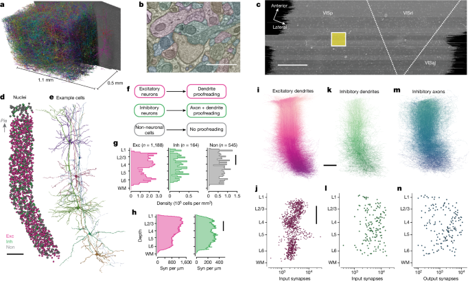
The second dataset covers a millimetre-square cross-sectional area, and 50 µm of depth within the primary visual cortex of a P49 male mouse18,20,51. The largest available segment spans the entire cortex through to layer 6. After applying the nuclear detection model18 and filtering out all nuclear objects below 25 µm3 and cells that were cut off by the volume border (see the section above entitled Filtering procedure), 1,944 cells were used for the analysis. The class type of each cell was labelled manually and used as the ground truth. Owing to the thinness of the volume, much of the distal cell morphologies were cut off and thus subclass type labelling was not possible. Nuclear and somatic mesh cleaning and feature extraction and normalization followed the same procedures.

The column borders were found by manually identifying a region in primary visual cortex that was far from both dataset boundaries and the boundaries with higher-order visual areas. The y axis of the dataset was extended along the basis of layer 2 and 100 100 m box.

The arbour’s radial extent. We define ‘radial distance’ to be the distance in the same plane as the pial surface. For every neuron, we computed a pia-to-white-matter line, including slanted region in deep layers, passing through its cell body. We used the same depth for each skeleton’s radial distance to the white-matter line. The 97th percentile distance was defined as the radial extent of the neuron.

We used a similar method to remove the axon fragments that were merged onto the dendrites. The unbranched segments on the non-Akonal region of the skeleton were identified and computed with input synapse density. We defined a false merge as one with an input density less than 0.1 synaptic inputs per micrometre, if the terminal segments had no downstream segments. This process iterated across terminal segments until all remaining had an input density of at least 0.1 inputs per micrometre. All segments were masked from the skeleton for analysis.

The expert neuroanatomists have grouped the excitatory and inhibitory neurones into subclasses. The thickness of the nucleus was compared to nuclear staining to figure out how much the cell body density is near the expected layer boundaries.

MICrONS: hierarchical neural network classification for the prediction of nucleus and synaptic input from a large sample of neurons

Owing to high levels of proofreading in the column, there were very few errors; thus, the training set was augmented with manually labelled errors from the entire dataset.

For measuring the synaptic output budget across cell types across the dataset (that is, inside and outside the column), we used a hierarchical classifier on the basis of a collection of perisomatic features that was trained on the data-driven clustering from the column sample40. Only synapses onto object segmentation associated with a single nucleus and a cell type classification were used. Almost all of the other targets were not Proofread, but that doesn’t mean they aren’t accurate.

A voxel participation in a nucleus was predicted by a cloud based network. The methods described in ref are followed. A nucleus prediction map was made on the entire dataset.

To measure the predicted cell densities per subclass across the MICrONS dataset, we divided the dataset into 50-µm2 bins in the x–z plane. We scaled the number of cells in each subclass to correspond to the number of square millimetre in the literature.

To determine if a cell preferentially Targeted 5P-NP neurons, we measured the fraction of total output that Targeted various predicted subclasses. Cells that produce a high proportion of their synapses onto the 5P-NP cells were considered to have this rare preference. A two-tailed Fisher exact test was carried out to test significance between the random cell population and the nearest neighbours.

To characterize the distribution of synaptic inputs relative to the cell body instead of cortical space, we computed the number of synapses in 13 soma-adjusted depth bins starting 100 µm above and below the soma. We computed the top five components using SparsePCA as before, and the synapse counts were Z-scored. The loadings for each of these components were used as further features.

The hierarchical model was defined as the sequential combination of the best-performing classifiers at each level. At each level of the hierarchy, see the Extended Data Table 1 for a snapshot of the different feature sets. The overall performance of the hierarchical model was measured with a test set that involved manual inspection of 100 examples of each of the neuronal and non-neuronal subclasses as well as errors. This resulted in a test set of 1,700 cells. The Hierarchical model has cross-validation and test performance reported. Note that all scores reported are the weighted accuracy based on the sampling rate of each class within the column.

The model type was picked based on a randomized grid search for the following models: support machine with a linear line, support machine with a radial line, nearest neighbours, Random forest and Neural network. For each type, 50 models were trained with varying parameters and the top-performing model was chosen. Individual models were further adjusted using a measure of recall called the F1 score. Training and test examples were held consistent across models for direct performance comparison within each level.

To build a descriptor that reflects the various properties of the PSS was the goal for the cell which all PSSs have been removed from. In particular, we aim to capture two of these properties: the type of shape of the PSS and the distance of the PSS from the soma. Moreover, as different cells can have different numbers of shapes (synapses), we needed a fixed-size representation for each cell. A dictionary of all shape types was built using the information from 236,000 PSSs. The shapes were normalized to train a Point Net autoencoder to learn a representation of size 1,024. The high-dimensional latent space spanning all of these shapes is a continuous space (Extended Data Fig. 3), which was used to generate a bag of words model30 for the shapes. To ensure that we were sampling the entire embedding space, we carried out k-means clustering with k = 30 to estimate cluster centres. The bincentres were manually rearranged for visualization purposes from the shapes that represented small spines, to the different shapes that acted like long spines, and finally the somatic compartments. The right panel has the top row. 4d shows the shape in the dictionary that is closest to each of these cluster centres. For distance from the soma, we split the 60 µm radius around the nucleus centre into four 15-µm radial bins (Fig. 4c,d). A histogram of counts was created from the binned PSSs’ shape and distance properties. Initially we extracted PSSs from within 120 µm radius. However, on inspection of the normalized histograms and the 2D UMAP embedding space, the additional radial bins did not increase our differentiability and did increase truncation effects near the dataset; thus, we reduced the radius to 60 µm. Finally, this histogram was z-scored and then added to the rest of the features as input to classifiers and the UMAP embedding (Figs. 4 and 6).

To rapidly skeletonize dynamic data, we took advantage of the PyChunkedGraph data structure that collects all supervoxels belonging to the same neuronal segmentation into 2 × 2 × 20 µm ‘chunks’ with a unique ID and precisely defined topological adjacency with neighbouring chunks of the same object. Each chunk is called a ‘level 2 chunk’, and the complete set of chunks for a neuron and their adjacency we call the ‘level 2 graph’ on the basis of its location in the hierarchy of the PyChunkedGraph data structure27. We precompute and cache a representative central point in space and the volume and the surface area for each level 2 chunk and update this data when new chunks are created because of proofreading edits. Using the level 2 graph and assigning edge lengths corresponding to the distance between the representative points for each vertex (that is, each level 2 chunk), we run the TEASAR75 algorithm (10 µm invalidation radius) to extract a loop-free skeleton. Each of the level 2 vertices removed by the TEASAR algorithm is associated with its closest remaining skeleton, making it possible to map surface area and volume data to the skeleton. New skeletons can be computed in about 10 days, making them useful for analysis over long scales of up to 100 micrometres.

For 2D UMAP embeddings and training of the classifiers, it was important to place all features in approximately similar scales. For this reason, we independently z-scored each feature across all cells and used that as the input for classifier training as well as the UMAP embeddings in Figs. 3–6.

MET-type predictions for inhibitory neurons from patch-seq and EM data: subclass classifications and a comparison of differentially expressed genes

A MET-type prediction was made for each inhibitory neuron from a defined 100 µm × 100 µm cortical column (these cells are analysed in greater detail in ref. 33). Given the diverse population of interneurons captured in these data and the Sst-centric focus of this paper, the data are presented at the subclass level (apart from Extended Data Fig. 4, which shows Patch-seq and EM morphologies mapped to Sst MET-types or non-Sst subclasses). Subclass labels were assigned based on MET-type classifications (for example, all Pvalb MET-types are categorized under the Pvalb subclass).

We analysed differentially expressed genes using scrattch.hicat (https://github.com/AllenInstitute/scrattch.hicat/tree/master) on the reference fluorescence-activated cell sorting-collected single-cell RNA sequencing dataset6 to compare the main transcriptomic types that make up each MET-type (MET-8: Ssthpse Cbln4 and MET-4 are related. Sst Calb2 Necab1and Calb2 Pdlim5 is the Sst. Sst cyla3 and Sst cyla2 Ptdg4 have been added. Sst Myh8 Etv. Pairwise differentially expressed genes were identified as previously described6 using the limma package69 and selecting genes with at least a twofold change in expression and an adjusted P value of less than 0.01. The top five upregulated and downregulated genes for each pairwise comparison were selected for visualization (ranked by adjusted P value). The average expression of these genes and the fraction of cells with non-zero expression was calculated for the neurons of the three Sst MET-types in the Patch-seq data16 and presented as a dot plot. Only genes expressed in half of the cells in a specific MET-type were selected for visualization.

The recently published MERFISH dataset67 estimates the proportion of MET types. The cell counts were calculated for each t-type. The cell types in the MERFISH database were mapped to a whole-brain t-type and the MET-types were based on a VISp-specific type. Correspondences between the original taxonomy of Tasic et al.6 and the cortex or hippocampal formation (CTX/HPF) taxonomy were identified by finding the Tasic et al.6 t-types that had the highest number of shared cells for each CTX/HPF t-type68. The correspondences from the whole-brain taxonomy were taken directly from the ref. 67. We have assigned Tasic et al.6 t-types to the MET-types that have the highest number of cells, except for the t-type Sst Calb2 Pdlim5 which has corresponding cells. Note that cells from the Sst Chodl subclass (Sst MET-1) were not analysed here. In addition, no clear t-type correspondences were identified for the MET-type Sst MET-11, which also contained a small number of cells in the original study16.

Using automatically detected synapses, annotators visualized all output synapses on a given presynaptic cell in Neuroglancer. Regions lacking synapses were manually inspected in the EM imagery. If myelination was seen, an annotator marked the start and end point of each myelinated segment in Neuroglancer to generate a line. The number of myelinated segments per cell was deduced from the number of annotations summed. The distance of axon per cell is determined by summing the length of the annotations.

For 500 iterations, a random subsample (95%) of the Patch-seq data was selected with probabilities according to MET-type class size (a Patch-seq cell from a well-represented MET-type was more likely to be omitted). The MET-types with five or fewer had not been included in the subsampling. In each iteration, a new RFC with the parameters was fitted with data and MET labels were predicted for EM cells. The final MET assignment was given as the most frequently predicted MET label for each cell (Extended Data Table 1). Group cells were analyzed using the predicted MET-type labels.

The mean and percentile of the Patch-seq data was used to calculate the z scores.

A reliability metric was calculated based on the fraction of iteration each sample was predicted as its final assignment out of all predictions, for example 80% of the time. To determine an appropriate threshold, we explored reliability scores in the Patch-seq data. We applied random subsampling iterations in a leave-one-out manner to the Patch-seq data. Here we set one Patch-seq sample aside and use the rest as training data. In each iteration, the training data are sub-sampled randomly as described above and used to fit a new RFC. The classifier predicts the MET-type label of the single left-out Patch-seq sample. Every Patch-seq cell had to be repeated 500 times before it had a predicted MET-type label and corresponding reliability metric. We then plotted a cumulative histogram of the correctly and incorrectly predicted labels versus the reliability score. We found that a reliability score of more than 0.54 is the most inclusive value at which Patch-seq samples are more frequently predicted correctly than incorrectly (Extended Data Fig. 2b).

An RFC, support vector machine and logistic regression model were assessed for performance in predicting MET-type labels for Patch-seq cells using the morphological features of inhibitory cell types from a previously published Patch-seq dataset (Patch-seq n = 477, Sst n = 236, Pvalb n = 89, Vip n = 79, Lamp5 n = 44, Sncg n = 29)16. The fivefold cross-validation approach was used to assess classification accuracy. The distribution of MET type labels in each partition remained the same while the data was split randomly. This method iteratively rotates partition so it’s not used for training. MET-types that had less than five reconstructions were not included. A maximum depth of ten, balanced class weights, a minimum of ten samples per split, and a minimum of five samples per leaf were all superior to support machine models for anRFC with 250 estimators. Fivefold stratified cross-validation with shuffling was repeated 20 times and achieved a mean accuracy of 58.9 ± 4.1% (s.e.m.), far exceeding the expected chance accuracy for 22 categories (4.5%). The model’s accuracy is determined by how often the model correctly predicted the MET label of held out data. 5a). We calculated an overall F1 score of 0.58, based on averaging F1 scores for each MET-type, based on classifying that type versus any other type. The cumulative confusion matrix for hold-out validation data was recorded in Fig. 1c.

The number of distinct branches of a neuron as a function of its distance to the soma and the median of schoons

We measured the number of distinct branches as a function of the distance from the soma, starting at 30 m and continuing to 300 m. For robustness relative to precise branch point locations, the number of branches were computed by finding the number of distinct connected components of the skeleton found in the subgraph formed by the collection of vertices between each distance value and 10 µm towards the soma. We computed the top three singular value components of the matrix on the basis of branch count versus distance for all excitatory neurons, and the loadings were used as features.

Because the fraction of synapses targeting all compartments sums to one, the last remaining property, synapses onto distal basal dendrites, was not independent and thus was measured but not included as a feature. Inspection of the data suggested two more properties that characterized synaptic output across inhibitory neurons:

A multisynaptic connection is a subset of the singlesynaptic connection, which includes at least two of the same pre and target neurones.

We applied a linear discriminant classifier to all the inhibitory cells and trained it using these six features. The differences between manual annotations and data were not treated as classifications but as a different view of data.

Median tortuosity of the path from branch tips to soma per cell. Tortuosity is measured as the ratio of path length to the Euclidean distance from tip to soma centroid.

There is a linear density of schoons. This was measured by computing the net path length and number of synapses along 50 depth bins from layer 1 to white matter and computing the median. A linear density was found by dividing synapse count by path length per bin, and the median was found across all bins with non-zero path length.

Source: Inhibitory specificity from a connectomic census of mouse visual cortex

The importance of each feature for each inhibitory M-type from a connectomic census of mouse visual cortex using scikit-learn78

All features were computed after a rigid rotation of 5 degrees to flatten the pial surface and translation to set the pial surface to 0 on the y axis. Features on the basis of apical classification were not explicitly used to avoid ambiguities on the basis of both biology and classification.

To compute the importance of each feature for each M-type, for each M-type we trained a random forest classifier to predict whether a cell belonged to it using scikit-learn78. Because the classes were strongly imbalanced, we used SMOTE resampling to oversample datapoints from the smaller class. We used the Mean Decrease in Impurity metric, which quantifies how often a given feature was used in the decision tree ensemble.

For the inhibitory motif group clustering, for each interneuron we first computed the number of synapses across each excitatory M-types in the column. This synaptic output budget was then normalized per cell to generate a vector for each neuron with elements ranging from zero to one. Normalized synaptic output budgets were oversegmented using k-means (k = 20) with Euclidean distances 500 times, and a matrix of coclustering frequency—that is, the number of times two cells were put in the same k-means cluster—between individual cells was computed. Final M-types were found through agglomerative clustering with complete linkage of the coclustering matrix, scanning from two to 25 output clusters and selecting a final value of 18 on the basis of silhouette score and Davies–Bouldin score.

On connectivity cards, we also show a similar selectivity index on the basis of compartment rather than M-type. In that case, the shuffled distribution preserves observed depth and M-type output distributions but not compartments.

Source: Inhibitory specificity from a connectomic census of mouse visual cortex

Auto-Tessellation of Mammalian Blood Vessels: Predicting the Clefts of the Presynaptic Partners

A network was created to predict whether a voxel took part in a synaptic cleft. Inference on the entire dataset was processed using the methods described in ref. The images are 8 8 40 x 40. The components that were removed from the predictions were smaller than 40 voxels. A network was trained to predict the voxels of the synaptic partners using an attentional signal. This assignment network was run for each detected cleft, and coordinates of both the presynaptic and postsynaptic partner predictions were logged along with each cleft prediction.

The alignment process is not likely to have an affect on the curvature as it is not aligned to a sectioning plane.

Blood vessel segmentation does not show a large, correlated distortion in deep layers, making it unlikely to be a result of mechanical stress on the tissue (https://ngl.microns-explorer.org/#!gs://microns-static-links/mm3/blood_vessels.json). It’s not clear why stress would affect only layer 5b and below.

In other large EM datasets, there have been similar phenomena, particularly among the layer 6 pyramidal cells.

The volume assembly pipeline is described in detail elsewhere62,63. Briefly, the images collected by the autoTEMs are first corrected for lens distortion effects using nonlinear transformations computed from a set of 10 × 10 highly overlapping images collected at regular intervals. Point correspondences can be derived using features from the scale-invariant feature transform. If you want to minimize the amount of squared distances between the tile images, you have to estimate the transform parameters per image. A per-section transformation is estimated by using a down sample version of these sections. The rough aligned volume is rendered to disk for further fine alignment. The AllenInstitute has a software tool to help you stitch and align the dataset. To fine align the volume, we needed to make the image processing pipeline robust. Cracks larger than 30 um (in 34 sections) were corrected by manually defining transforms. The smaller cracks and folds in the dataset were automatically identified using a type of computer software called a convolutional network, that trained on manually labelled samples. The same was done to identify voxels containing tissue. The alignment was refined using a coarse-to-fine hierarchy and a convolutional network to estimate displacements between images. The images were further transformed when displacement fields were estimated between sections to create a final field for each image. The first step in refining alignment was using 1,024 1,024 40 nm3 images. The composite image of the partial sections was created using the tissue mask previously computed.

The parallel imaging pipeline used in this study61 used a fleet of transmission electron microscopes that had been converted to continuous automated operation. It was built on a standard JEOL 1200EXII 120 KHz transmission electron microscope, which had been modified with custom hardware and software. A low-distortion lens was used to grab image frames at 100 ms for a single large-format camera. The autoTEM also provided fast, high-fidelity montaging of large tissue sections, as well as a reel-to-reel tape translation system to locate each section using index barcodes. During imaging, the reel-to-reel GridStage moved the tape and located the targeting aperture through its barcode and acquired a 2D montage. We performed quality control on all image data and reimaged sections that failed the screening.

The candidate mice were shipped via overnight air freight from the college of Medicine to the Allen Institute. Mice were transcardially perfused with a fixative mixture of 2.5% paraformaldehyde, 1.25% glutaraldehyde and 2 mM calcium chloride, in 0.08 M sodium cacodylate buffer, pH 7.4. A thick (1,200 µm) slice was cut with a vibratome and post-fixed in perfusate solution for 12–48 h. Slices were extensively washed and prepared for reduced osmium treatment based on the protocol of ref. 64. All steps were performed at room temperature, unless indicated otherwise. The first osmication step involved 2% osmium tetroxide (78 mM) with 8% v/v formamide (1.77 M) in 0.1 M sodium cacodylate buffer, pH 7.4, for 180 min. 90 min was given to reduce the osmium after use of the 75 mM of Potassium ferricyanide. The second osmium step was at a concentration of 2% in 0.1 M sodium cacodylate for 150 min. Samples were washed with water and then immersed in thiocarbohydrazide for further intensification of the staining (1% thiocarbohydrazide (94 mM) in water, 40 °C, for 50 min). After washing with water, samples were immersed in 2% water for 90 minutes. After extensive washing in water, Walton’s lead aspartate (20 mM lead nitrate in 30 mM aspartate buffer, pH 5.5, 50 °C, 120 min) was used to enhance contrast. After two rounds of washes, the samples went through a graded dehydration series, consisting of 50%, 70%, and 10% w/v in water, 30 min each at 4C, then 3 100%, 30 min each at room temperature. Two rounds of 100% acetonitrile (30 min each) served as a transitional solvent step before proceeding to epoxy resin (EMS Hard Plus). A progressive resin infiltration series (1:2 resin:acetonitrile (for eample, 33% v/v), 1:1 resin:acetonitrile (50% v/v), 2:1 resin acetonitrile (66% v/v) and then 2 × 100% resin, each step for 24 h or more, on a gyrotary shaker), was done before final embedding in 100% resin in small coffin moulds. Epoxy was cured at 60 °C for 96 h before unmoulding and mounting on microtome sample stubs. The sections were collected at a minimum thickness of 40 NM with the aid of a modified ATUMtome.

The Allen Institute for Brain Science has an Institutional Animal Care and Use Committee. Neurophysiology data acquisition was conducted at Baylor College of Medicine before EM imaging. After being moved to the Allen Institute in Seattle, the mice were kept in a facility for up to 3 days where they were euthanized and perfused. All results described here are from a single male mouse, age 64 days at onset of experiments, expressing GCaMP6s in excitatory neurons via SLC17a7-Cre and Ai162 heterozygous transgenic lines (recommended and generously shared by Hongkui Zeng at the Allen Institute for Brain Science; JAX stock 023527 and 031562, respectively). Two-photon functional and structural scanning of the cells and vessels took place between P75 and P80. The mouse was removed from its body.

Source: Inhibitory specificity from a connectomic census of mouse visual cortex

The MICrONS Dataset. Part I: Acquisition, Alignment, Segmentation and Primary Resource (extended abstract)

This dataset was acquired, aligned and segmented as part of the larger MICrONS project. Methods underlying dataset acquisition are described in full detail elsewhere2,61,62,63, and the primary data resource is described in a separate publication2. The methodological details we repeat here for convenience were used in the dataset.