The wet and dry season are the result of rainforest destruction in the area

Read Time:3 Minute, 51 Second

Importance of Amazonian deforestation on precipitation reverses between seasons: comparison of simulated and satellite data at 20-km resolution

To validate the spatial variability of surface air temperature and precipitation, the monthly accumulated precipitation from the WRF simulations was compared with satellite records at a 20-km resolution. We resampled four rainfall datasets, for which the original resolutions are finer than 20 km, at a resolution of 20 km for validation. The results indicated that our model generally captured the spatial patterns of monthly precipitation during the wet and dry seasons (Extended Data Fig. 6). During the wet season, precipitation in the Amazon region is complex with our simulations capturing spatial patterns compared with satellite data aligning with the diagonal line and showing a correlation coefficients of 0.48 to 0.56 6a–d. During the dry season, the results indicate strong spatial relationships between the simulated and satellite-recorded precipitation (R values ranging from 0.80 to 0.87, P < 0.01) (Extended Data Fig. 6e–h.

You can say that it’s a speach of $$rmrain_rmtrmormd.

Source: Impact of Amazonian deforestation on precipitation reverses between seasons

Assessing the impact of Amazon deforestation on precipitation in 2000-2020 using high-resolution 20-km resolution GLAD data

There are two scenarios for forest cover, one representing land cover and the other forest cover changes in 2000. The percentages of non-forest categories went up for grid cells with net forest losses, and they went down for forest categories. Conversely, in grid cells with net forest gain, the percentages of forest categories increased proportionally, whereas the percentages of non-forest categories decreased. The S 2020 scenario maintained the same proportion among five forest cover types as in 2000, varying only in total forest cover percentage. After we derived the deforestation scenario (S2020) over the whole domain, we substituted the land cover and land use fraction of the Amazon region with MODIS land cover in 2000 and obtained the S2000 scenario. The results of S2020 minus S2000 are shown in the main text. The influence of the model boundary was assessed during a simulation of wet and dry seasons under the larger model domain.

In this study, climate modelling and the moving window approach were used to quantify the precipitation impacts of Amazon deforestation. The methods have differences in their assumptions and strengths. 8). For climate modelling, we can obtain the comprehensive impacts of deforestation and further explore the local and nonlocal effects on buffers at different scales. For the moving window approach using satellite-observed datasets, the realistic impact of deforestation on precipitation can be quantified. However, this quantification is limited to deforested pixels, and the effects on neighbouring and remote pixels cannot be quantified. When a de forested piece is compared with a de forested piece, the intrinsic effects are ignored. We compared the methods using model simulations and satellite observations.

We used high-resolution (30 m) forest cover data for 2000 and 2020 from the Global Land Analysis and Discovery (GLAD) forest extent and height change dataset22,23 to resample forest cover change information at a 20-km resolution (Extended Data Fig. 1c. GLAD forest cover data from 2000 and 2020 were mapped by attributing pixels with forest height ≥5 m as the ‘forest’ land cover class, which agrees with the definition of ‘forest’ by the Food and Agriculture Organization of the United Nations. We derived forest cover changes by comparing the years 2000 and 2020, defining ‘deforestation’ as grid cells in which forest cover decreased from 2000 to 2020 at a 20-km resolution.

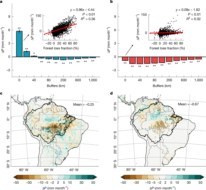
A two side student t-test was used to determine whether the distributions of mean precipitation effects are different from zero. Moreover, we conducted a more rigorous field significance test using the Benjamini–Hochberg method to control the false discovery rate (FDR) at α = 0.05. The results highlight model grids that have local significant P values and remain significant after FDR correction. Linear regression is used to fit the relationship between forest loss fraction and ΔP over deforested grids. The Wald test is used to see if the hypothesis that the slope is zero is true.

The frontier of current research, therefore, lies in advancing analytical frameworks, such as the one presented by Qin et al., by coupling them with dynamic modelling of vegetation. Only when the interacting effects of climate change, deforestation and vegetation health are linked can the risk of tipping be truly assessed. As with the work of Qin et al., consideration of seasonal as well as dry and warm extremes will be important steps in this process.