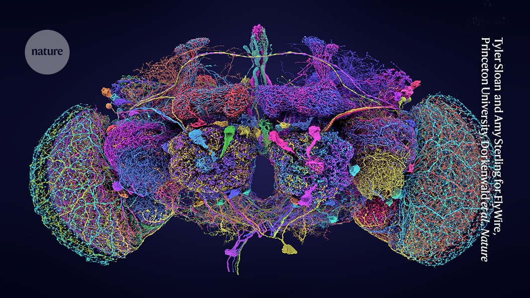
The biggest brain map ever reveals the fruit fly’s neurons

Analytical Estimation of the Dimensionality of the KC Activities in the Connectomic Dataset and the FlyWire CAmAID Project

There are only two values in the matrix, either 0 or 1 and. In a way, this helps when calculating analytical results for the dimensionality of the KC activities. The data from connectomics shows the number of synaptic connections between the KCs and the ALPNs.

The linear rate model in the original paper is not known if it represents the behavior of the biological neural circuit well. Furthermore, it remains unproven that the ALPN-KC neural circuit is attempting to maximize the dimensionality of the KC activities, albeit the theory is biologically well motivated (but see refs. 49,50).

To avoid the bias, we used a fraction of the total synaptic budget for the cell types we were looking at in the KC analysis. The fraction of APL output that is spent on each of the different KC types was examined. In other words, we quantified the cost for individualKCs as a fraction of the population’s budget.

The true number of inputs onto a given neurons is typically lower than the reported counts. The free-floating fragments in the dataset can not be joined onto the rest of the neuron because of fine-calibre fragments.

The dataset published by Buhmann et al. contained ~244 million synapses. We removed synapses from the imported list if they fulfilled any of the following criteria: (1) either the pre- or postsynaptic location remained unassigned to a segment (proofread or unproofread); (2) It had a score ≤50. The annotations between the same pre- and postsynaptic partners were removed because they were too close to each other. We were left with a total of 130 million synapses.

There is a publicly available version of the FlyWire CAmAID project. This project uses a new extension that allows users to create and administer their own tracing environments on top of the publicly available neuronal image volumes and connectomic datasets. Users can use the ORCiD public authentication service to log in to public CATMAID projects. Users can create their own copies of public projects. The user becomes administrator and can invite other users to join him in this new project. Invitations are managed through project tokens, which the administrator can generate and send to invitees for access to the project. There is a way to load data from the dedicated FAFB-FlyWire server in the more general Spaces environment.

When a matched type was either missing large parts of its arbours due to truncation in the hemibrain or the comparison with the FlyWire matches suggested closer inspection was required, we used cross-brain connectivity comparisons (see the section below) to decide whether to adjust (split or merge) the type. A merge of two or more hemibrain types was recorded, and the split was recorded with a lower case letter as a suffix. In rare cases in which we were able to find a match for an untyped hemibrain neuron, we would record the hemibrain body ID as hemibrain type and assign a CBXXXX identifier as cell type.

Cell types that exist only on the left but not the right hemisphere of the hemibrain because our comparison was principally against the right hemisphere.

Skeletization of Neuron Meshes for a Robust Morphological Analysis of Early-Borne Neurons

Our companion paper (149.2 m) included high-resolution skeletons that could be used to calculate the length of the neuronal cable. In brief, we downloaded neuron meshes (LOD 1) from the flat 783 segmentation (available at gs://flywire_v141_m783) and skeletonized them using the wavefront method implemented in skeletor (https://github.com/navis-org/skeletor). After being re-stomp to their Soma, they were smoothed, healed, and a bit down sampled due to segmentation issues. A modified version of this pipeline is implemented in fafbseg. You can download skeletons through the Data availability and Code availability sections.

To test the robustness of the morphological groups, we reran the above analysis across one, two or three hemispheres. This treatment sometimes gave slightly different results. However, some groups of neurons consistently co-clustered across the different hemispheres; we termed these ‘persistent clusters’. Early-born neurons, which are often distinct, frequently failed to participate in clusters, and were omitted from further analysis. We used two- and three-hemisphere clustering to link these persistent clusters, for example, the TuBu neurons from both the left and right hemispheres would fall. Morphological groups are therefore defined by consistent across-hemisphere clustering. When neurons of a given hemilineage were sufficiently contained by the hemibrain volume, all three hemispheres (two from FlyWire and one from hemibrain) were used; otherwise, the two hemispheres from FlyWire were used. As we prioritized consistency across 1, 2 and 3 hemisphere clustering, a minority of neurons with a hemilineage annotation do not have a morphological group. For example, if neuron type A clusters with type B in one-hemisphere clustering, but clusters with type C (and not B) in two-hemisphere clustering, then type A will not have a morphological group annotation.

For FlyWire, we re-used the dotprops generated for the all-by-all NBLAST (see the previous section). The points outside the hemibrain bounding box were removed to account for the truncation of the hemibrain volume.

Before the NBLAST, we additionally transformed dotprops to the same side by mirroring those from neurons with side right onto the left. If the matrix was symmetrical, we could use min(A + AT) to generate minimum scores for the NBLAST.

Hierarchical annotation and multi-connectome cell typing of Drosophila: The hemibra is a complex system with several classes of intransic neurons

The central brain has Cell classes that represent groupings that were used in the literature. The class indicates the level of the sensory neuronal activity. For optic-lobe-intrinsic neurons cell class indicates their neuropil innervation: for example, cell class ‘ME’ are medulla local neurons, ‘LA>ME’ are neurons projecting from the lamina to the medulla and ‘ME>LO.LOP’ are neurons projecting from the medulla to both lobula and lobula plate.

Hierarchical annotations include flow, superclass, class (plus a subclass field in certain cases) and cell type. The flow and superclass were generally assigned based on an initial semi-automated approach followed by extensive and iterative manual curation. See Supplementary Table 3 for definitions and the sections below for details on certain superclasses.

Biological outliers range from small additional/missing branches to entire misguided neurite tracks, and were typically assessed within the context of a given cell type and best possible contralateral matches within FlyWire and/or the hemibrain. When biological outliers were suspected, careful proofreading was undertaken to avoid erroneous merges or splits of neuron segmentation.

Some neurons can’t be traced due to a main neurite suddenly ends, so they are missing large arbours. In crowded areas, a lot of neurites cross the brain’s midline. We were able to bridge the gaps, and find the missing branch, by using left–right matching. We marked them as outliers where they remained incomplete.

Source: Whole-brain annotation and multi-connectome cell typing of Drosophila

Enhanced box plots for the FlyWire map: a python analysis of the statistical significance and the neuronal inhibition

Enhanced box plots—also called letter-value plots125—in Fig. 5h and Extended Data Fig. 7f are a variation of box plots better suited to represent large samples. They replace the whiskers with a variable number of letter values where the number of letters is based on the uncertainty associated with each estimate, and therefore on the number of observations. The ‘fattest’ letters are the (approximate) 25th and 75th quantiles, respectively, the second fattest letters the (approximate) 12.5th and 87.5th quantiles and so on. The underlying data is unrelated to the width of the letters.

The data from the FlyWire map can be explored by researchers. This has enabled scientists to learn more about the brain and about fruit flies — findings that are captured in some of the papers published in Nature today.

Statistical analyses were performed using the methods in the scipy123 python package. To determine statistical significance, we used either t-tests for normally distributed samples, or Kolmogorov–Smirnov tests otherwise.

The number of input connections to each mixing layer neuron is kept at a constant K for all neurons. It is definitely a simplification that can be corrected by introducing a distribution P(K) but this requires further detailed modelling.

The global inhibition given to all of the mixing layer neurons is assumed to take a single value. If there are more APL and mixing layer neurones, the level of inhibition would be different.

A Digital Mirror for FAFB-FlyWire Data: Neuronal Assignments, Sensory Annotations, and Neural Categorization

From Fig. The shift from higher values of K in the model to lower values in the FlyWire left and FlyWire right dataset show how the model works.

For consistency with visualizations and datasets obeying the standard convention (fly’s right on viewer’s left), FlyWire data can be mirrored. Using the Python flybrains and natverse nat.jrcbrains, we are able to digitally mirror FAFB-FlyWire data. Through 1c.

Our reconstruction used the FAFB electron microscopy dataset9. A number of consortium members noticed that the images seemed to be inverted for the asymmetric body123. Eventually a left–right inversion during FAFB imaging was confirmed. The true biological side is what determines the side annotations in figures. For technical reasons, we were unable to invert the underlying FAFB image data and therefore continue to show images and reconstructions in the same orientation as in Zheng et al.9, although we now know that in such frontal views the fly’s left is on the viewer’s left. For full details of this issue including approaches to display FAFB and other brain data with the correct chirality, please see the companion paper12.

The companion paper contains descriptions of nerve assignments, sensory annotations, and neural categorization. In brief, neurons were assigned to one of three ‘flow’ classes: afferent (to the brain), intrinsic (within the brain) and efferent (out of the brain). The arbor was within the FlyWire brain dataset. This included cells that projected to and from the SEZ. Next, each flow class was divided into superclasses in the following way. afferent: sensory, ascending. intrinsic: central, optic, visual projection (from the optic lobes to the central brain), visual centrifugal (from the central brain to the optic lobes). Efferent is the endocrine, descending motor.

ANs were identified based on the following criteria: (1) no soma in the brain; and (2) main branch entering through the neck connective (note that some ANs make a dendrite after entry through the neck connective and then an axon).

To identify what is described in the ref. In the EM dataset, we made the volume rendering of the DN GAL4 lines into FlyWire space. Matching of closely related neurons can be done by displaying the same space for both EM andLFMs. For DNs without available volume renderings, we identified candidate EM matches by eye, transformed them into JRC2018U space and overlaid them onto the GAL4 or Split GAL4 line stacks (named in ref. 107 for that type) in FIJI for verification. Using these methods, we identified all but two (DNd01 and DNg25) in FAFB/FlyWire and annotated their cell type with the published nomenclature. All of the unmatched DNs received a systematic cell type consisting of their soma location, an e for EM type and a three digit number. A detailed account and analysis of DNs has been published108 separately.

Besides the canonical root point, the soma position was recorded for all neurons with a cell body. This was either based on curating entries in the nucleus segmentation table (removing duplicates or positions outside the nucleus) or on selecting a location, especially when the cell body fibre was truncated and no soma could be identified in the dataset. These soma locations were critical for a number of analyses and also allowed a consistent side to be defined for each neuron. This was done by defining left and right with a cutting plane at the middle line of the mediolateral (x) axis. The soma positions within 20 m of the plane were manually reviewed. The goal was to define a consistent logical soma side based on examination of the cell body fibre tracts entering the brain; this ultimately ensured that cell types present, for example, in one copy per brain hemisphere, were always annotated so that one neuron was identified as the left and the other the right. In a small number of cases, for example, for the bilaterally symmetric octopaminergic ventral unpaired medial neurons, we assigned side as ‘central’.

For sensory neurons, side refers to whether they enter the brain through the left or the right nerve. In a small number of cases we could not unambiguously identify the nerve entry side and assigned side as ‘na’.

Neurons can have both a cell_type and a hemibrain_type entry, in which case, the cell_type represents a refinement or correction and should take precedence. A total of 8,453 terminal cell types are reported in this report, with 3,662 hemibrain-derived cell types and 4,581 new types included. New types consist of 3,504 CBXXXX types, 65 new visual centrifugal neuron types (‘c’ prefix, for example, cL08), 173 new VPN types (‘e’ suffix, for example, LTe07), 602 new AN types (‘AN_’ or ‘SA_’ prefix, for example, AN_SMP_1) and 237 new DN types (‘e’ suffix, for example, DNge094). The remaining 229 types are cell types known from other literature, for example, columnar cell types of the optic lobes.

We give cell type annotations for > 92% of the brain’s cells. The majority of these types are based on previous literature. We started the typing effort by annotating well-known large tangential cells (for example, Am1 or LPi12), VPNs (for example, LT1s) as well as photoreceptor neurons. We followed a number of different strategies, sometimes in combination, for the neurons with known fingerprints and the downstream or upstream of them. (2) We ran connectivity clustering as described above on both optic lobes combined. There were clusters reviewed and matched against literature. Each round added or refined new cell types to inform the next round of clustering. We were able to match some of the clusters against the previously described cell types, but not all of them.

Johnston’s organ neurons in the right hemisphere were characterized based on innervation of the major AMMC zones (A, B, C, D, E and F), but not further classified into subzone innervation as shown previously104. Other sensory cells in the right hemisphere include taste peg, gustatory, and mechanosensory bristle cells. Through their interaction with the uniglomerular projection neurons, olfactory, and hygrosensory cells of the antennal lobes were identified.

Sensory neuron were also cross-referenced to existing literature to assign cell types through the class field. The left hemisphere has almost all head mechanosensory bristle and taste peg, found in the right hemisphere. Gustatory sensory neurons were previously identified in ref. 103 and Johnston’s organ neurons in refs. 104,105 in a version of the FAFB that used manual reconstruction (https://fafb.catmaid.virtualflybrain.org). Those neurons were identified in the FlyWire instance by transformation and overlay onto FlyWire space as described previously102.

Re-ranching provisional cell types of VCNs using hemibrain clustering: the case of SLPp3/BLVa2c, Pb1/CM6, SLP1pl2,CP6, PSp

The majority of VCNs were assigned to specific types. There were 29 VPNs and 9 VCNs that could not be confidently assigned a cell type.

To validate a subset of the new, provisional cell types, we re-ran the clustering using three hemispheres (FlyWire + hemibrain) on 25 cross-identified hemilineages that are not truncated in the hemibrain (Extended Data Fig. 9). The procedure was the same as for double-clustering.

For VPNs the nomenclature follows the format [neuropil][C/T][e][XX], where neuropil refers to regions innervated by VPN dendrites; C/T denotes columnar versus tangential organization; e indicates identification through EM; and XX represents a zero padded two digit number.

We assigned neuropils to the left and right hemispheres or the centre if the neuropil has no homologue. We then counted how many postsynapses each neuron had in each of these three regions and assigned it to the one with the largest count.

By comprehensively inspecting the hemilineage tracts originally in CATMAID and then in FlyWire, we can now reconcile previous reports. It’s new to refs. These are the neurons that we gave the lineage. 33,34. New to ref. They are named: SLPpl3/BLVa2c, Pb1/CM6, SLPpl2,CP6, PSp. The following clones were not taken from ref. It is necessary to account for the total number of lineages/hemilineages because they don’t seem to have been clearly demonstrated in the larva.

There are light-level clones from refs. 33,34 match very well the great majority of the time, sometimes clones with the same name only match partially. For example, the AOTUv1_ventral/DALcm2_ventral hemilineage seems to be missing in the AOTUv1/DALcm2 clone in the Ito collection33. There appears to be a similar situation for the DM4/CM4, EBa1/DALv2 and LHl3/BLVa2b lineages. When there is a conflict, we have preferred clones as described in ref. 34.

This pipeline is implemented in the coconatfly package (Table 1), which provides a streamlined interface to carry out such clustering. The following command will allow you to examine if the types given to a selection of neurons are robust.

An optional interactive mode allows for efficient exploration within a web browser. You can see more examples and details at www.natverse.org/coconatfly.

On the Dimensionality of Responses of Large KCs to Interactions. II. The Effect of Double Checking of the Hemibrain Types

In rare cases, the hemibrain types were double checked and corrected, for example by merging two or more hemibrain types, or removing hemibrain type labels.

How it changes with respect to the number of connections. In other words, what are the numbers of input connections K onto individual KCs that maximize the dimensionality of their responses, h, given M KCs, N ALPNs and a global inhibition α?

More detailed calculations can be found in a previous report122. Randomized and homogeneous weights were used to populate ({\bf{W}}), such that each row in ({\bf{W}}) has K elements that are 1 − α and N − K elements that are −α. The parameter α represents a homogeneous inhibition corresponding to the biological, global inhibition by APL. The value inhibition was set to be α = A/M, where A = 100 is an arbitrary constant and M is the number of KCs in each of the three datasets. The primary amount of interest is the size of the activities.

Distributed Proofreading of the FlyWire Release 783: Evaluation and Estimates of Timescales During Early Releases of the Neuronal Wiring Diagram

The professional proofreading team received additional proofreading training. Correct proofreading relies on a diverse array of 2D and 3D visual cues. Proofreaders learned about 3D morphology, resulting from false merger or false split without knowing what types of cells they are. Ultrastructures have various types and are useful guides for accurate tracing. Before professional proofreaders were admitted into Production, each of them practiced on average >200 cells in a testing dataset where additional feedback was given. We compared the test cells to ground-truth reconstructions to determine their accuracy. To improve proofreading quality, peer learning was highly encouraged.

Any quantification of the total proofreading time that was required to create the FlyWire resource is a rough estimate because of the distributed nature of the community, the interlacing of analysis and proofreading and the variability in how proofreading was performed. The second public release, version 783, required 3,013,513 edits. We measured proofreading times during early proofreading rounds that included proofreading of whole cells in the central brain. A total of 29,135 independent proofread tasks were edited after outliers were removed. We were able to get an average time for edits from the data. However, we observed that proofreading times per edit were much higher for proofreading tasks that required few edits (<5). The second round of proofreader went over all segments with >100synaptics, meaning our measurements were not representative. These are usually required edits. We adjusted for that by computing estimates for proofreading speeds of both rounds by limiting the calculations to a subset of the timed tasks: (round 1) The average time per edit in our proofreading time dataset, (round 2) the average time of tasks with 1–5 edits. In order to get an overall proofreading time, we averaged the times for the tasks in each category. The result was an average time of 79 s per edit which adds up to an estimate of 33.1 person-years assuming a 2,000 h work year.

FlyWire uses CAVE50 to host its annotations. The PyChunkedGraph is part of CAVE’s proofreading system.

Source: Neuronal wiring diagram of an adult brain

The Hemibra: a Neuropil Comparison of the Completion Rates and Synapse Numbers for 9 Neurons

We assigned synapses to neuropils based on their presynaptic location. We used the nCOllpyde project to determine if the location was inside a neuropil mesh and assign the synapse accordingly. Some synapses remained unassigned after this step because the neuropils only resemble rough outlines of the underlying data. We placed all remaining synapses to the closest one if they were within 10 m. The rest of the synapses were left unassigned.

We calculated a volume for each neuropil using its mesh. In the aggregated volumes presented in the paper we assigned the lamina, medulla, accessory medulla, lobula and lobula plate to the optic lobe. The ocellar ganglion was assigned to the central brain.

R,fracrmTPrmTP+rmFP,.

We retrieved the latest completion rates and synapse numbers for the hemibrain from neuprint (v1.2.1). There may be cases where a neuropil comparison can’t be directly possible because of the changes in the hemibrain dataset. We did not include these regions in the comparison.

The brain can be defined as a ring-shaped structure that is extended from the pharynx to the excretory area. (We follow the authors who call this region the nerve ring plus the anterior portion of the ventral nerve cord, though some authors refer to the combined structure as the nerve ring.) Nine neurons (RIR, RIV, RMDD, RMD and RMDV) are intrinsic to the nerve ring itself. There are an extra 26 neurons that are in the combined structure of the brain.

It should be understood that this estimate has ‘error bars’ because of definitional ambiguities. Ten motor neurons (RMH, RMF and RMD) could arguably be removed from the list, as it is unclear whether motor neurons qualify as intrinsic neurons. The brain could be enlarged by moving the border further behind the excretory pore, with the addition of ten neurons. 3510 intrinsic neuron are estimated to make these ambiguities explicit. Of the 302 CNS neurons, 180 make synapses in the brain126. Therefore, neurons intrinsic to the brain make up about 15 to 25% of brain neurons, and 8 to 15% of CNS neurons.

We used L2Cache50 to figure out the cell volumes and surface areas. Volumes were computed by counting all voxels within a cell segment and multiplying the count by the voxel resolution. The area calculations were more complicated because they had overlap through shifts in space. We shifted the binarized segment in each dimension individually and extracted the overlap of false and true voxels. For each dimension, we counted the extracted voxels and multiplied the count by the voxel resolution of the given dimensions. Finally, we added up the per dimensions area estimates. The measurement was too compute intensive and it will overrepresent the area slightly.

The synapse classifier by Buhmann et al. was trained on ground truth from the CREMI challenge (https://cremi.org). There are 3 5 5 5 m cubes from the calyx in FAB14 in the three CREMI datasets. They looked at the classifier’s performance on multiple regions after it was trained and validation on only this dataset. It should be noted that performance varies by region.

Eckstein et al.10 created a machine learning model to predict neurotransmitter identities for all synapses from Buhmann et al. based on the electron microscopy imagery alone. The probabilities were assigned for all the neurotransmitters, and each one was assigned a probability. They used theneurotransmitter identities published for individual cell types to build a dataset, assuming Dale’s law applies. A per-Synapse accuracy of 80% and a per neuron accuracy of 98% were reported by the authors.

For each neuron, we calculated the fraction of presynapses in the left and right hemisphere. The hemisphere opposite its dominant input side was named the contralateral hemisphere. Most of the postsynapses in the centre region are not included.

We used the information flow algorithm implemented by Schlegel et al.26,128 (https://github.com/navis-org/navis) to calculate a rank for each neuron starting with a set of seed neurons. The graph of neurons are mapped out in a probabilistic way. The likelihood of a neuron being added to the traversed set increased linearly with the fraction of synapses it receives from already traversed neurons up to 30% and was guaranteed above this threshold. We repeated the rank calculation for all the sensory neurons as well as their seeds. The groups we used are: olfactory receptor neurons, gustatory receptor neurons, mechanosensory Johnston’s organ neurons, head and neck bristle mechanosensory neurons, mechanosensory taste peg neurons, thermosensory neurons, hygrosensory neurons, VPNs, visual photoreceptors, ocellar photoreceptors and ascending neurons.

Input seeds were created by combining all of the listed options and having visual sensory groups excluded.

For each modality we performed 10,000 runs, which were averaged. We then ordered the neurons according to their rank and assigned them a percentile based on their location in the order. We used UMAP129 to compute a reduceddimensionality by putting all ranks into a neuron and using the min_dist and metric to calculate twodimensional embeddings.

The FlyWire project: Connecting brain cells to one another: A discovery of 581 new neuronal cell types based on an annotated wiring diagram

But these tools aren’t perfect, and the wiring diagram needed to be checked for errors. The scientists spent a great deal of time manually proofreading the data — so much time that they invited volunteers to help. In all, the consortium members and the volunteers made more than 3 million manual edits, according to co-author Gregory Jefferis, a neuroscientist at the University of Cambridge, UK. He notes that a large amount of this work took place in 2020 when fly researchers were at a loss as to what to do with themselves.

The team was surprised by some of the ways in which the various cells connect to one another, too. For instance, neurons that were thought to be involved in just one sensory wiring circuit, such as a visual pathway, tended to receive cues from multiple senses, including hearing and touch1. “It’s astounding how interconnected the brain is,” Murthy says.

But the work wasn’t finished: the map still had to be annotated, a process in which the researchers and volunteers labelled each neuron as a particular cell type. Humans would need to check the results of any artificial intelligence trained to recognize lakes and roads in satellite images before they could name the specific lakes or roads. The researchers identified more types of neuron than they had expected. Of these, 4,581 were newly discovered, which will create new research directions, Seung says. He says every one of those celltypes is a question.

The map1 is described in a package of nine papers about the data published in Nature today. Its creators are part of a consortium known as FlyWire, co-led by neuroscientists Mala Murthy and Sebastian Seung at Princeton University in New Jersey.

“This is a huge deal,” says Clay Reid, a neurobiologist at the Allen Institute for Brain Science in Seattle, Washington, who was not involved in the project but has worked with one of the team members who was. “It’s something that the world has been anxiously waiting for, for a long time.”