The regime has changed in the sea ice thickness
Calving fronts of ZI and NG: long term evolution using GIPSY-OASIS with JPL data processing and atmospheric delay models
We used aerial and satellite images to map the calving fronts of ZI and NG over a period of 10 years. For ZI, the most notable changes occurred between 2011 and 2013, when a large portion of its floating extension collapsed, resulting in a retreat of 10 km (ref. 53). This collapse has been followed by a steady retreat of about 700 m year−1. After large sections of its floating tongue were lost from 2002 to 2004, the calving events on the main floating tongue have been less frequent. More than 120 km2 of floating shelf ice was released into the ocean in 2020 due to the northern section of theNG collapsing.
We process the GNSS data using the GIPSY-OASIS software package with high-precision kinematic data processing methods27 and with ambiguity resolution using the orbit and clock products of the Jet Propulsion Laboratory (JPL). GIPSY-OASIS version 6.4 was developed at the JPL 30. JPL final orbit products include satellite clock parameters and Earth orientation parameters. The orbit products take the satellite antenna phase centre offsets into account. The atmospheric delay parameters are modelled using the Vienna Mapping Function 1 (VMF1) with VMF1 grid nominals54. Solid Earth tide and ocean tidal loading can be removed with a correction. The FES-2014b ocean tide model uses the Automatic Load Provider to calculate the phases and amplitudes of the main ocean tidal loading terms. The site coordinates are computed through the IGS14 frame55. We convert the Cartesian coordinates at 15-s intervals into local up, north and east coordinates for each GNSS site monitored at the NEGIS surface. The example of a 15-s solution is in the Extended Data fig. 2c–c.
For the last 3 decades, sea ice trajectories have been calculated in order to investigate changes of pathways and residence time. Eight pseudo-ice floes were settled in the western half of the Fram Strait section (from prime meridian to 10° W) at the same time and advected backwards in time. On the 15th of every month, the calculations began. Daily sea ice motion vectors from the NSIDCv4 were used to update daily position of ice floes backwards in time. The ice motion plots at the different areas were then calculated by taking the surrounding points and adding them to an e-folding scale of 25 km. 6 years ago, the trajectory calculation was done, but it was called off if a sea ice concentration of 15% or less was available. The sea ice concentration at the ice encrusted position was obtained from OSI-409/OSI-430, which has a folding scale of 25 km. The position of each trajectory termination was used to define the location of ‘initial sea ice formation’. The analysis was not used because thejectories shorter than three months were excluded.
The flow acceleration is corrected at NEG1 and NEG2 in order to compensate for the downhill movement of the gis stations.
Extended Data Fig. The same information is presented in 4c. 4b but for the point P2, which is located at about 1,078 m elevation. The annual signal is 0.08 m in this location.
We use the best-fitting seventh-order polynomial (such as the red curve in Extended Data Fig. 4d,e) for each location shown in Extended Data Fig. 4a to estimate the annual rates of elevation changes from April to April, for example, from April 2011 to April 2012, from April 2012 to April 2013 etc.
We don’t merger NASA’s ATM surveys with other satellites when we create elevation time series. Instead, we estimate the annual elevation change rates from April to April for each dataset independently and then merge the rates.
The data shows an example of elevation changes at the overlap points. There is a noticeable elevation change near the glacier margin.
We correct the observed ice surface elevations for bedrock movement caused by elastic uplift owing to present-day mass changes and long-term past ice changes (glacial isostatic adjustment (GIA)). We correct for GIA using the GNET-GIA empirical model61. We put together an estimate of the dhGIA and uncertainty for each grid point. We correct for the elastic uplift of the bedrock by taking ice loss estimates from CryoSat-2 and ICESat-2 and using them to derive the Green’s functions. For each grid point, we estimate the elastic uplift rate dhelas and the associated uncertainty σelas. The elevation change rate for each grid point is
The model we use is the ice-sheet and Sea-level System Model, or ISSM63. The horizontal mesh resolution varies from 200 m near the ice front to 20 km inland, and it is vertically extruded into four layers. The model is based on a 3D higher-order approximation of the full Stokes model to include vertical shear for the stress balance; this is a good approximation for both fast-moving and slow-moving regions64,65. The surface and bed geometry from BedMachine Greenland50 has been used. The ice viscosity is determined by floats and conditions under grounded ice. We use the Budd friction law and slope to figure out the initial conditions. We calculate the friction coefficients for a regularized Coulomb law to produce the same stress. The friction coefficient is kept constant in time during the simulations. The choice of a law can have a significant impact on simulations. However, here we select the friction law based on observations.
There are models that are able to reproduce deep inland acceleration. Therefore, the choice of friction laws is reduced to the regularized Coulomb friction law and the Budd friction law with exponents of 1/5 and 1/6, as all the other models were unable to generate deep inland acceleration.
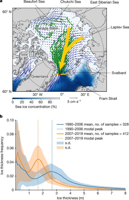
Dynamic sea ice thickening associated with dynamic ice deformation from upward looking sonar moorings in the western Fram Strait
Sea ice draft data were obtained from upward looking sonar (ULS) moored in the East Greenland Current in the western Fram Strait. The last three decades have some short temporal gaps. Four ULSs were zonally aligned at approximately 79° N from 3° W to 6.5° W (Fig. 1a). The latitude of the mooring array changed from 79° N to 78.8° N in 2001. Three of the moorings have ZOMIC positions of 3 W (F11), 4 W (F12), and 5 W (F13). There are three main temporal data gaps during the three decades of measurements, that is, 1996, 2002 and 2008. Despite the differences in their number, ULSs were still in operation. The travel time of the sound reflecting at the bottom of the sea ice is calculated by using the ice draft, the underwater fraction of sea ice54. The raw data were processed to ice draft using procedures described in earlier literature55,56. The accuracy of each draft measurement ranges from 0.1 m (ice profiling sonars (IPS) deployed after 2006) to 0.2 m (ES300 instruments before 2006), while the uncertainty of each individual measurement is not subject to bias errors and the summary error statistics of monthly values are less than 0.1 m57.
frac1sqrt2rmpi limits acute
In this study, we provide a concept and description of a stochastic model that formulates sea ice thickening associated with dynamic ice deformation. The model formulates three features of dynamic sea ice thickening by ridging and/or rafting: (1) dynamic ice thickening is a stochastic process (areal and thickening stochasticity); (2) thicker ice has a larger potential to get thicker than thinner ice at a dynamic event (proportionate ice thickening); and (3) thinner ice has a higher probability of dynamic deformation due to its weaker ice strength (preferential deformation of thinner over thicker ice types). The first point consists of two types of stochasticity in the dynamic ice thickening process. One is areal stochasticity, corresponding to the fact that ice deformation only occurs for a small fraction of the pack ice while the rest of the ice is unchanged when a dynamic event occurs. The other is thickening stochasticity, representing the fact that the thickness gain by ridging/rafting varies in space and differs between events. The second point represents a sea ice characteristic that thicker ice is tolerant and can exert stronger compressive force on the ice forming ridges and/or rafts; hence, more energy is potentially available for the dynamic thickening30,31. The thinner part of the pack ice is preferentially ridged/rafted when there is a dynamic event. This also takes into account the effect of ice thickness changes on the dynamic thickening process, for example, the thinner ice condition in recent years increases the likelihood of ice deformation.
Source: https://www.nature.com/articles/s41586-022-05686-x
A model of ice-pack fracturing by cyclones and the number of dynamic events for ln am and X0
where (\acute{X}(m)={e}^{\nu m}) and (\acute{\sigma }(m)=\sigma {m}^{1/2}) and ν and σ2 are the mean and variance of the population distribution of ln am (including X0), respectively67.
$${a}{i}=\left{\begin{array}{cc}1+b{r}{i} & {\rm{w}}{\rm{i}}{\rm{t}}{\rm{h}}\,{\alpha }{i}({\rm{ \% }})\,{\rm{p}}{\rm{r}}{\rm{o}}{\rm{b}}{\rm{a}}{\rm{b}}{\rm{i}}{\rm{l}}{\rm{i}}{\rm{t}}{\rm{y}}\ 1 & {\rm{w}}{\rm{i}}{\rm{t}}{\rm{h}}\,1-{\alpha }{i}({\rm{ \% }})\,{\rm{p}}{\rm{r}}{\rm{o}}{\rm{b}}{\rm{a}}{\rm{b}}{\rm{i}}{\rm{l}}{\rm{i}}{\rm{t}}{\rm{y}}\end{array}\right.$$
Another parameter necessary for the model is the number of dynamic events, m, that is, external forcing that could cause mechanical fracturing of sea ice and consequent ridging and/or rafting. We used the number of Arctic cyclones that passes over the ice pack as a first-order indicator of the number of dynamic events. Typically 90–130 cyclones per year occur in the Arctic Ocean (40–60 cyclones in winter, 50–70 cyclones in summer)71. A typical size of a Hurricane is roughly 106 km2 and covers approximately one third of the ice-covered area of the Indian Ocean. We therefore assumed that one-third of all cyclones hits the ice pack at a certain location in the Arctic, that is, the ice pack experiences approximately 40 dynamic events per year. For the typical residence time of sea ice in the high latitudes, 80–200 dynamic events are associated with this.
The ice is a coefficient of ice growth. This term comes from a simplified thermodynamic process without thermal inertia of sea ice and heat flux from the ocean72: